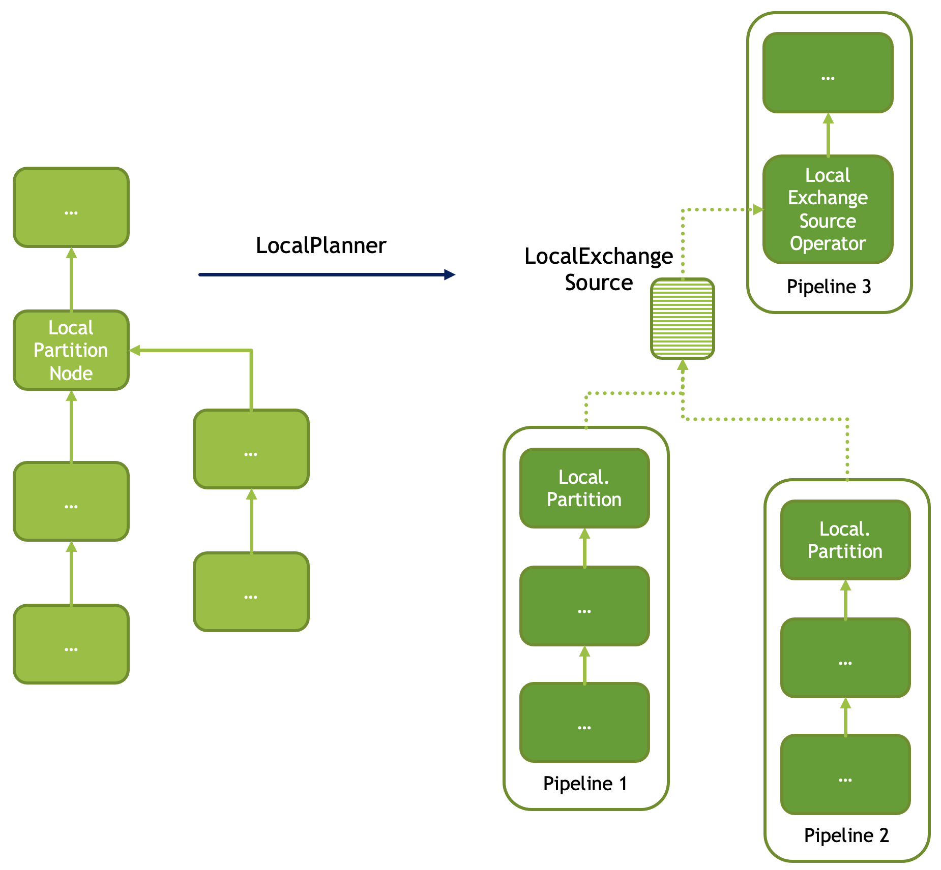
Plan Nodes and Operators

Velox query plan is a tree of PlanNode’s. Each PlanNode has zero or more child PlanNode’s. To execute a query plan, Velox converts it into a set of pipelines. Each pipeline is made of a linear sequence of operators that corresponds to a linear sub-tree of the plan. The plan tree is broken down into a set of linear sub-trees by disconnecting all but one child node from each node that has two or more children.

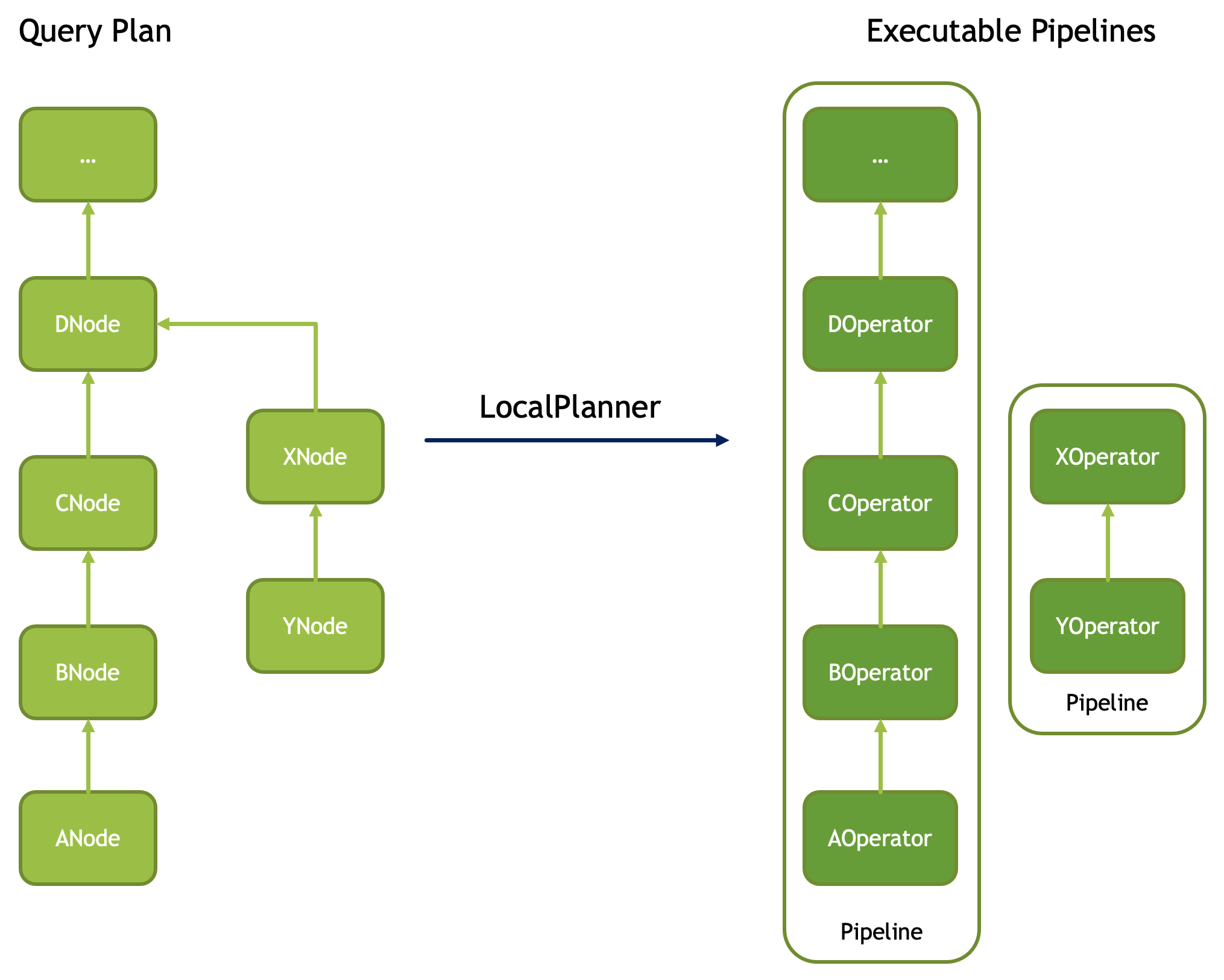
The conversion of plan nodes to operators is mostly one-to-one. Some exceptions are:

• Filter node followed by Project node is converted into a single operator FilterProject

• Nodes with two or more child nodes are converted to multiple operators, e.g. HashJoin node is converted to a pair of operators: HashProbe and HashBuild.

Operators corresponding to leaf nodes are called source operators. Only a subset of plan nodes can be located at the leaves of the plan tree. These are:

• TableScanNode

• ValuesNode

• ExchangeNode

• MergeExchangeNode

• ArrowStreamNode

Here is a list of supported plan nodes and corresponding operators.

Plan Node	Operator(s)	Leaf Node / Source Operator
TableScanNode	TableScan	Y
ArrowStreamNode	ArrowStream	Y
FilterNode	FilterProject
ProjectNode	FilterProject
AggregationNode	HashAggregation or StreamingAggregation
GroupIdNode	GroupId
MarkDistinctNode	MarkDistinct
HashJoinNode	HashProbe and HashBuild
MergeJoinNode	MergeJoin
NestedLoopJoinNode	NestedLoopJoinProbe and NestedLoopJoinBuild
OrderByNode	OrderBy
TopNNode	TopN
LimitNode	Limit
UnnestNode	Unnest
TableWriteNode	TableWrite
TableWriteMergeNode	TableWriteMerge
PartitionedOutputNode	PartitionedOutput
ExchangeNode	Exchange	Y
ExpandNode	Expand
MergeExchangeNode	MergeExchange	Y
ValuesNode	Values	Y
LocalMergeNode	LocalMerge
LocalPartitionNode	LocalPartition and LocalExchange
EnforceSingleRowNode	EnforceSingleRow
AssignUniqueIdNode	AssignUniqueId
WindowNode	Window
RowNumberNode	RowNumber
TopNRowNumberNode	TopNRowNumber

Plan Nodes

TableScanNode

The table scan operation reads data from a connector. For example, when used with HiveConnector, table scan reads data from ORC or Parquet files.

Property	Description
outputType	A list of output columns. This is a subset of columns available in the underlying table. The order of columns may not match the schema of the table.
tableHandle	Connector-specific description of the table. May include a pushed down filter.
assignments	Connector-specific mapping from the table schema to output columns.

ArrowStreamNode

The Arrow stream operation reads data from an Arrow array stream. The ArrowArrayStream structure is defined in Arrow abi, and provides the required callbacks to interact with a streaming source of Arrow arrays.

Property	Description
arrowStream	The constructed Arrow array stream. This is a streaming source of data chunks, each with the same schema.

FilterNode

The filter operation eliminates one or more records from the input data based on a boolean filter expression.

Property	Description
filter	Boolean filter expression.

ProjectNode

The project operation produces one or more additional expressions based on the inputs of the dataset. The project operation may also drop one or more of the input columns.

Property	Description
names	Column names for the output expressions.
expressions	Expressions for the output columns.

AggregationNode

The aggregate operation groups input data on a set of grouping keys, calculating each measure for each combination of the grouping keys. Optionally, inputs for individual measures are sorted and de-duplicated.

Property	Description
step	Aggregation step: partial, final, intermediate, single.
groupingKeys	Zero or more grouping keys.
preGroupedKeys	A subset of the grouping keys on which the input is known to be pre-grouped, i.e. all rows with a given combination of values of the pre-grouped keys appear together one after another. The input is not assumed to be sorted on the pre-grouped keys. If input is pre-grouped on all grouping keys the execution will use the StreamingAggregation operator.
aggregateNames	Names for the output columns for the measures.
aggregates	One or more measures to compute. Each measure specifies an expression, e.g. count(1), sum(a), avg(b), optional boolean input column that’s used to mask out rows for this particular measure, optional list of input columns to sort by before computing the measure, an optional flag to indicate that inputs must be deduplicated before computing the measure. Expressions must be in the form of aggregate function calls over input columns directly, e.g. sum(c) is ok, but sum(c + d) is not.
ignoreNullKeys	A boolean flag indicating whether the aggregation should drop rows with nulls in any of the grouping keys. Used to avoid unnecessary processing for an aggregation followed by an inner join on the grouping keys.
globalGroupingSets	If the AggregationNode is over a GroupIdNode, then some groups could be global groups which have only GroupId grouping key values. These represent global aggregate values.
groupId	GroupId is the grouping key in the AggregationNode for the groupId column generated by an underlying GroupIdNode. It must be of BIGINT type.

Properties of individual measures.

Property	Description
call	An expression for computing the measure, e.g. count(1), sum(a), avg(b). Expressions must be in the form of aggregate function calls over input columns directly, e.g. sum(c) is ok, but sum(c + d) is not.
rawInputTypes	A list of raw input types for the aggregation function. There are used to correctly identify aggregation function, e.g. to decide between min(x) and min(x, n) in case of intermediate aggregation. These can be different from the input types specified in ‘call’ when aggregation step is intermediate or final.
mask	An optional boolean input column that’s used to mask out rows for this particular measure. Multiple measures may specify same input column as a mask.
sortingKeys	An optional list of input columns to sort by before computing the measure. If specified, sortingOrders must be used to specify the sort order for each sorting key.
sortingOrders	A list of sorting orders for each sorting key.
distinct	A boolean flag indicating that inputs must be de-duplicated before computing the measure.

Note that if measures specify sorting keys, HashAggregation operator accumulates all input rows in memory before sorting these and adding to accumulators. This requires a lot more memory as compared to when inputs do not need to be sorted.

Similarly, if measures request inputs to be de-duplicated, HashAggregation operator accumulates all distinct input rows in memory before adding these to accumulators. This requires more memory as compared to when inputs do not need to be de-duplicated.

Furthermore, many aggregate functions produce same results on sorted and unsorted inputs, e.g. min(), max(), count(), sum(). The query planner should avoid generating plans that request sorted inputs for such aggregate functions. Some examples of aggregate functions that are sensitive to the order of inputs include array_agg() and min_by() (in the presence of ties).

Similarly, some aggregate functions produce same results on unique inputs as well as inputs with duplicates, e.g. min(), max(). The query planner should avoid generating plans that request de-duplicating inputs for such aggregate functions.

Finally, note that computing measures over sorted input is only possible if aggregation step is ‘single’. Such computations cannot be split into partial + final.

To illustrate the need for globalGroupingSets and groupIdColumn, we examine the following SQL

SELECT orderkey, sum(total_quantity) FROM orders GROUP BY CUBE (orderkey);

This is equivalent to the following SQL with GROUPING SETS

SELECT orderkey, sum(total_quantity) FROM orders GROUP BY GROUPING SETS ((orderkey), ());

The SQL gives sub-totals of total_quantity for each orderkey along with the global sum (from the empty grouping set).

The optimizer plans the above query as an Aggregation over a GroupId node.

Lets say the orders table has 5 rows:

orderkey   total_quantity
   1            5
   2            6
   2            7
   3            8
   4            9

After GroupId for the grouping sets ((orderkey), ()) the table has the following 10 rows

orderkey   total_quantity    group_id
   1            5                0
   2            6                0
   2            7                0
   3            8                0
   4            9                0
   null         5                1
   null         6                1
   null         7                1
   null         8                1
   null         9                1

A subsequent aggregation with grouping keys (orderkey, group_id) gives the sub-totals for the query

orderkey   total_quantity     group_id
  1           5                  0
  2           13                 0
  3           8                  0
  4           9                  0
  null        35                 1

If there were no input rows for this GROUP BY CUBE, then the expected result is a single row with the default value for the global aggregation. For the above query that would be:

orderkey   total_quantity      group_id
  null           null             1

To generate this special row the AggregationNode needs the groupId for the global grouping set (1 in this case) and it returns a single row for it with the aggregates default value.

Note: Presto allows multiple global grouping sets in a single SQL query.

SELECT orderkey, sum(total_quantity) FROM orders GROUP BY GROUPING SETS ((), ());

Hence, globalGroupingSets is a vector of groupIds.

ExpandNode

For each input row, generates N rows with M columns according to specified ‘projections’. ‘projections’ is an N x M matrix of expressions: a vector of N rows each having M columns. Each expression is either a column reference or a constant. Both null and non-null constants are allowed. ‘names’ is a list of M new column names. The semantic of this operator matches Spark. Using project and unnest can be employed to implement the expand functionality. However, the performance is suboptimal when creating an array constructor within the Project operation.

Property	Description
projections	A vector of N rows each having M columns. Each expression is either a column reference or a constant.
names	A list of new column names.

ExpandNode is typically used to compute GROUPING SETS, CUBE, ROLLUP and COUNT DISTINCT.

To illustrate how ExpandNode works lets examine the following SQL query:

SELECT l_orderkey, l_partkey, count(l_suppkey) FROM lineitem GROUP BY ROLLUP(l_orderkey, l_partkey);

In the planning phase, Spark generates an Expand operator with the following projection list:

[l_suppkey, l_orderkey, l_partkey, 0],
[l_suppkey, l_orderkey, null,      1],
[l_suppkey, null,       null,      3]

Note: The last column serves as a special group ID, indicating the grouping set to which each row belongs. In Spark, this ID is calculated using a bitmask. If a certain column is selected, the bit value is assigned as 0; otherwise, it is assigned as 1. Therefore, the binary representation of the first row is (000), resulting in 0. The binary representation of the second row is (001), resulting in 1. The binary representation of the third row is (011), resulting in 3.

For example, if the input rows are:

l_suppkey l_orderkey l_partkey
93        1          673
75        2          674
38        3          22

After the computation by the ExpandNode, each row will generate 3 rows of data. So there will be a total of 9 rows:

l_suppkey l_orderkey l_partkey grouping_id_0
93        1          673       0
93        1          null      1
93        null       null      3
75        2          674       0
75        2          null      1
75        null       null      3
38        3          22        0
38        3          null      1
38        null       null      3

Aggregation operator that follows, groups these 9 rows by (l_orderkey, l_partkey, grouping_id_0) and computes count(l_suppkey):

l_orderkey l_partkey count(l_suppkey)
1          673       1
null       null      3
1          null      1
2          null      1
2          674       1
3          null      1
3          22        1

Another example would be COUNT DISTINCT query.

SELECT COUNT(DISTINCT l_suppkey), COUNT(DISTINCT l_partkey) FROM lineitem;

In the planning phase, Spark generates an Expand operator with the following projection list:

[l_suppkey, null,      1],
[null,      l_partkey, 2]

For example, if the input rows are:

l_suppkey l_partkey
93        673
75        674
38        22

After the computation by the ExpandNode, each row will generate 2 rows of data. So there will be a total of 6 rows:

l_suppkey l_partkey grouping_id_0
93        null      1
null      673       2
75        null      1
null      674       2
38        null      1
null      22        2

Aggregation operator that follows, groups these rows by (l_suppkey, l_partkey, grouping_id_0) and produces:

l_suppkey l_partkey grouping_id_0
93        null      1
75        null      1
38        null      1
null      673       2
null      674       2
null      22        2

Another Aggregation operator that follows, computes global count(l_suppkey) and count(l_partkey) producing final result:

COUNT(DISTINCT l_suppkey) COUNT(DISTINCT l_partkey)
3                         3

GroupIdNode

Duplicates the input for each of the specified grouping key sets. Used to implement aggregations over grouping sets.

The output consists of grouping keys, followed by aggregation inputs, followed by the group ID column. The type of group ID column is BIGINT.

Property	Description
groupingSets	List of grouping key sets. Keys within each set must be unique, but keys can repeat across the sets. Grouping keys are specified with their output names.
groupingKeyInfos	The names and order of the grouping key columns in the output.
aggregationInputs	Input columns to duplicate.
groupIdName	The name for the group-id column that identifies the grouping set. Zero-based integer corresponding to the position of the grouping set in the ‘groupingSets’ list.

GroupIdNode is typically used to compute GROUPING SETS, CUBE and ROLLUP.

While usually GroupingSets do not repeat with the same grouping key column, there are some use-cases where they might. To illustrate why GroupingSets might do so lets examine the following SQL query:

SELECT count(orderkey), count(DISTINCT orderkey) FROM orders;

In this query the user wants to compute global aggregates using the same column, though with and without the DISTINCT clause. With a particular optimization strategy optimize.mixed-distinct-aggregations, Presto uses GroupIdNode to compute these.

First, the optimizer creates a GroupIdNode to duplicate every row assigning one copy to group 0 and another to group 1. This is achieved using the GroupIdNode with 2 grouping sets each using orderkey as a grouping key. In order to disambiguate the groups the orderkey column is aliased as a grouping key for one of the grouping sets.

Lets say the orders table has 5 rows:

orderkey
   1
   2
   2
   3
   4

The GroupIdNode would transform this into:

orderkey   orderkey1   group_id
1             null        0
2             null        0
2             null        0
3             null        0
4             null        0
null           1          1
null           2          1
null           2          1
null           3          1
null           4          1

Then Presto plans an aggregation using (orderkey, group_id) and count(orderkey1).

This results in the following 5 rows:

orderkey     group_id     count(orderkey1) as c
1                0         null
2                0         null
3                0         null
4                0         null
null             1          5

Then Presto plans a second aggregation with no keys and count(orderkey), arbitrary(c). Since both aggregations ignore nulls this correctly computes the number of distinct orderkeys and the count of all orderkeys.

count(orderkey)     arbitrary(c)
 4                     5

HashJoinNode and MergeJoinNode

The join operation combines two separate inputs into a single output, based on a join expression. A common subtype of joins is an equality join where the join expression is constrained to a list of equality (or equality + null equality) conditions between the two inputs of the join.

HashJoinNode represents an implementation that starts by loading all rows from the right side of the join into a hash table, then streams left side of the join probing the hash table for matching rows and emitting results.

MergeJoinNode represents an implementation that assumes that both inputs are sorted on the join keys and streams both join sides looking for matching rows and emitting results.

Property	Description
joinType	Join type: inner, left, right, full, left semi filter, left semi project, right semi filter, right semi project, anti. You can read about different join types in this blog post.
nullAware	Applies to anti and semi project joins only. Indicates whether the join semantic is IN (nullAware = true) or EXISTS (nullAware = false).
leftKeys	Columns from the left hand side input that are part of the equality condition. At least one must be specified.
rightKeys	Columns from the right hand side input that are part of the equality condition. At least one must be specified. The number and order of the rightKeys must match the number and order of the leftKeys.
filter	Optional non-equality filter expression that may reference columns from both inputs.
outputType	A list of output columns. This is a subset of columns available in the left and right inputs of the join. The columns may appear in different order than in the input.

NestedLoopJoinNode

NestedLoopJoinNode represents an implementation that iterates through each row from the left side of the join and, for each row, iterates through all rows from the right side of the join, comparing them based on the join condition to find matching rows and emitting results. Nested loop join supports non-equality join.

Property	Description
joinType	Join type: inner, left, right, full.
joinCondition	Expression used as the join condition, may reference columns from both inputs.
outputType	A list of output columns. This is a subset of columns available in the left and right inputs of the join. The columns may appear in different order than in the input.

OrderByNode

The sort or order by operation reorders a dataset based on one or more identified sort fields as well as a sorting order.

Property	Description
sortingKeys	List of one of more input columns to sort by.
sortingOrders	Sorting order for each of the soring keys. The supported orders are: ascending nulls first, ascending nulls last, descending nulls first, descending nulls last.
isPartial	Boolean indicating whether the sort operation processes only a portion of the dataset.

TopNNode

The top-n operation reorders a dataset based on one or more identified sort fields as well as a sorting order. Rather than sort the entire dataset, the top-n will only maintain the total number of records required to ensure a limited output. A top-n is a combination of a logical sort and logical limit operations.

Property	Description
sortingKeys	List of one of more input columns to sort by. Must not be empty and must not contain duplicates.
sortingOrders	Sorting order for each of the soring keys. See OrderBy for the list of supported orders.
count	Maximum number of rows to return.
isPartial	Boolean indicating whether the operation processes only a portion of the dataset.

LimitNode

The limit operation skips a specified number of input rows and then keeps up to a specified number of rows and drops the rest.

Property	Description
offset	Number of rows of input to skip.
count	Maximum number of rows to return.
isPartial	Boolean indicating whether the operation processes only a portion of the dataset.

UnnestNode

The unnest operation expands arrays and maps into separate columns. Arrays are expanded into a single column, and maps are expanded into two columns (key, value). Can be used to expand multiple columns. In this case produces as many rows as the highest cardinality array or map (the other columns are padded with nulls). Optionally can produce an ordinality column that specifies the row number starting with 1.

Property	Description
replicateVariables	Input columns that are returned unmodified.
unnestVariables	Input columns of type array or map to expand.
unnestNames	Names to use for expanded columns. One name per array column. Two names per map column.
ordinalityName	Optional name for the ordinality column.

TableWriteNode

The table write operation consumes one output and writes it to storage via a connector. An example would be writing ORC or Parquet files. The table write operation return a list of columns containing the metadata of the written data: the number of rows written to storage, the writer context information, the written file paths on storage and the collected column stats.

Property	Description
columns	A list of input columns to write to storage. This may be a subset of the input columns in different order.
columnNames	Column names to use when writing to storage. These can be different from the input column names.
aggregationNode	Optional Aggregation plan node used to collect column stats for the data written to storage.
insertTableHandle	Connector-specific description of the destination table.
outputType	A list of output columns containing the metadata of the data written storage.

TableWriteMergeNode

The table write merge operation aggregates the metadata outputs from multiple table write operations and returns the aggregated result.

Property	Description
outputType	A list of output columns containing the metadata of the written data aggregated from multiple table write operations.

PartitionedOutputNode

The partitioned output operation redistributes data based on zero or more distribution fields.

Property	Description
kind	Specifies output buffer types: kPartitioned, kBroadcast and kArbitrary. For kPartitioned type, rows are partitioned and each sent to corresponding destination partition. For kBroadcast type, rows are not partitioned and sent to all the destination partitions. For kArbitrary type, rows are not partitioned and each sent to any one of the destination partitions.
keys	Zero or more input fields to use for calculating a partition for each row.
numPartitions	Number of partitions to split the data into.g
replicateNullsAndAny	Boolean flag indicating whether rows with nulls in the keys should be sent to all partitions and, in case there are no such rows, whether a single arbitrarily chosen row should be sent to all partitions. Used to provide global-scope information necessary to implement anti join semantics on a single node.
partitionFunctionFactory	Factory to make partition functions to use when calculating partitions for input rows.
outputType	A list of output columns. This is a subset of input columns possibly in a different order.

ValuesNode

The values operation returns specified data.

Property	Description
values	Set of rows to return.
parallelizable	If the same input should be produced by each thread (one per driver).
repeatTimes	How many times each vector should be produced as input.

ExchangeNode

A receiving operation that merges multiple streams in an arbitrary order. Input streams are coming from remote exchange or shuffle.

Property	Description
type	A list of columns in the input streams.

MergeExchangeNode

A receiving operation that merges multiple ordered streams to maintain orderedness. Input streams are coming from remote exchange or shuffle.

Property	Description
type	A list of columns in the input streams.
sortingKeys	List of one of more input columns to sort by.
sortingOrders	Sorting order for each of the soring keys. See OrderBy for the list of supported orders.

LocalMergeNode

An operation that merges multiple ordered streams to maintain orderedness. Input streams are coming from local exchange.

Property	Description
sortingKeys	List of one of more input columns to sort by.
sortingOrders	Sorting order for each of the soring keys. See OrderBy for the list of supported orders.

LocalPartitionNode

A local exchange operation that partitions input data into multiple streams or combines data from multiple streams into a single stream.

Property	Description
Type	Type of the exchange: gather or repartition.
partitionFunctionFactory	Factory to make partition functions to use when calculating partitions for input rows.
outputType	A list of output columns. This is a subset of input columns possibly in a different order.

EnforceSingleRowNode

The enforce single row operation checks that input contains at most one row and returns that row unmodified. If input is empty, returns a single row with all values set to null. If input contains more than one row raises an exception.

Used for queries with non-correlated sub-queries.

AssignUniqueIdNode

The assign unique id operation adds one column at the end of the input columns with unique value per row. This unique value marks each output row to be unique among all output rows of this operator.

The 64-bit unique id is built in following way: - first 24 bits - task unique id - next 40 bits - operator counter value

The task unique id is added to ensure the generated id is unique across all the nodes executing the same query stage in a distributed query execution.

Property	Description
idName	Column name for the generated unique id column.
taskUniqueId	A 24-bit integer to uniquely identify the task id across all the nodes.

WindowNode

The Window operator is used to evaluate window functions. The operator adds columns for the window functions output at the end of the input columns.

The window operator groups the input data into partitions based on the values of the partition columns. If no partition columns are specified, then all the input rows are considered to be in the same partition. Within each partition rows are ordered by the values of the sorting columns. The window function is computed for each row at a time in this order. If no sorting columns are specified then the order of the results is unspecified.

Property	Description
partitionKeys	Partition by columns for the window functions.
sortingKeys	Order by columns for the window functions.
sortingOrders	Sorting order for each sorting key above. The supported sort orders are asc nulls first, asc nulls last, desc nulls first and desc nulls last.
windowColumnNames	Output column names for each window function invocation in windowFunctions list below.
windowFunctions	Window function calls with the frame clause. e.g row_number(), first_value(name) between range 10 preceding and current row. The default frame is between range unbounded preceding and current row.
inputsSorted	If true, the Window operator assumes that the inputs are clustered on partition keys and sorted on sorting keys in sorting orders. In this case, the operator splits the window partition and begins processing it as soon as it receives the data. If false, the Window operator accumulates all inputs first, then sorts the data, splits the window partition based on the defined criteria, and then processes each window partition sequentially.

RowNumberNode

An optimized version of a WindowNode with a single row_number function, an optional limit, and no sorting.

Partitions the input using specified partitioning keys and assigns row numbers within each partition starting from 1. The operator runs in streaming mode. For each batch of input it computes and returns the results before accepting the next batch of input.

This operator accumulates state: a hash table mapping partition keys to total number of rows seen in this partition so far. Returning the row numbers as a column in the output is optional. This operator doesn’t support spilling yet.

This operator is equivalent to a WindowNode followed by FilterNode(row_number <= limit), but it uses less memory and CPU and makes results available before seeing all input.

Property	Description
partitionKeys	Partition by columns.
rowNumberColumnName	Optional output column name for the row numbers. If specified, the generated row numbers are returned as an output column appearing after all input columns.
limit	Optional per-partition limit. If specified, the number of rows produced by this node will not exceed this value for any given partition. Extra rows will be dropped.

TopNRowNumberNode

An optimized version of a WindowNode with a single row_number function and a limit over sorted partitions.

Partitions the input using specified partitioning keys and maintains up to a ‘limit’ number of top rows for each partition. After receiving all input, assigns row numbers within each partition starting from 1.

This operator accumulates state: a hash table mapping partition keys to a list of top ‘limit’ rows within that partition. Returning the row numbers as a column in the output is optional. This operator doesn’t support spilling yet.

This operator is logically equivalent to a WindowNode followed by FilterNode(row_number <= limit), but it uses less memory and CPU.

Property	Description
partitionKeys	Partition by columns for the window functions. May be empty.
sortingKeys	Order by columns for the window functions. Must not be empty and must not overlap with ‘partitionKeys’.
sortingOrders	Sorting order for each sorting key above. The supported sort orders are asc nulls first, asc nulls last, desc nulls first and desc nulls last.
rowNumberColumnName	Optional output column name for the row numbers. If specified, the generated row numbers are returned as an output column appearing after all input columns.
limit	Per-partition limit. If specified, the number of rows produced by this node will not exceed this value for any given partition. Extra rows will be dropped.

MarkDistinctNode

The MarkDistinct operator is used to produce aggregate mask columns for aggregations over distinct values, e.g. agg(DISTINCT a). Mask is a boolean column set to true for a subset of input rows that collectively represent a set of unique values of ‘distinctKeys’.

Property	Description
markerName	Name of the output mask column.
distinctKeys	Names of grouping keys.

Examples

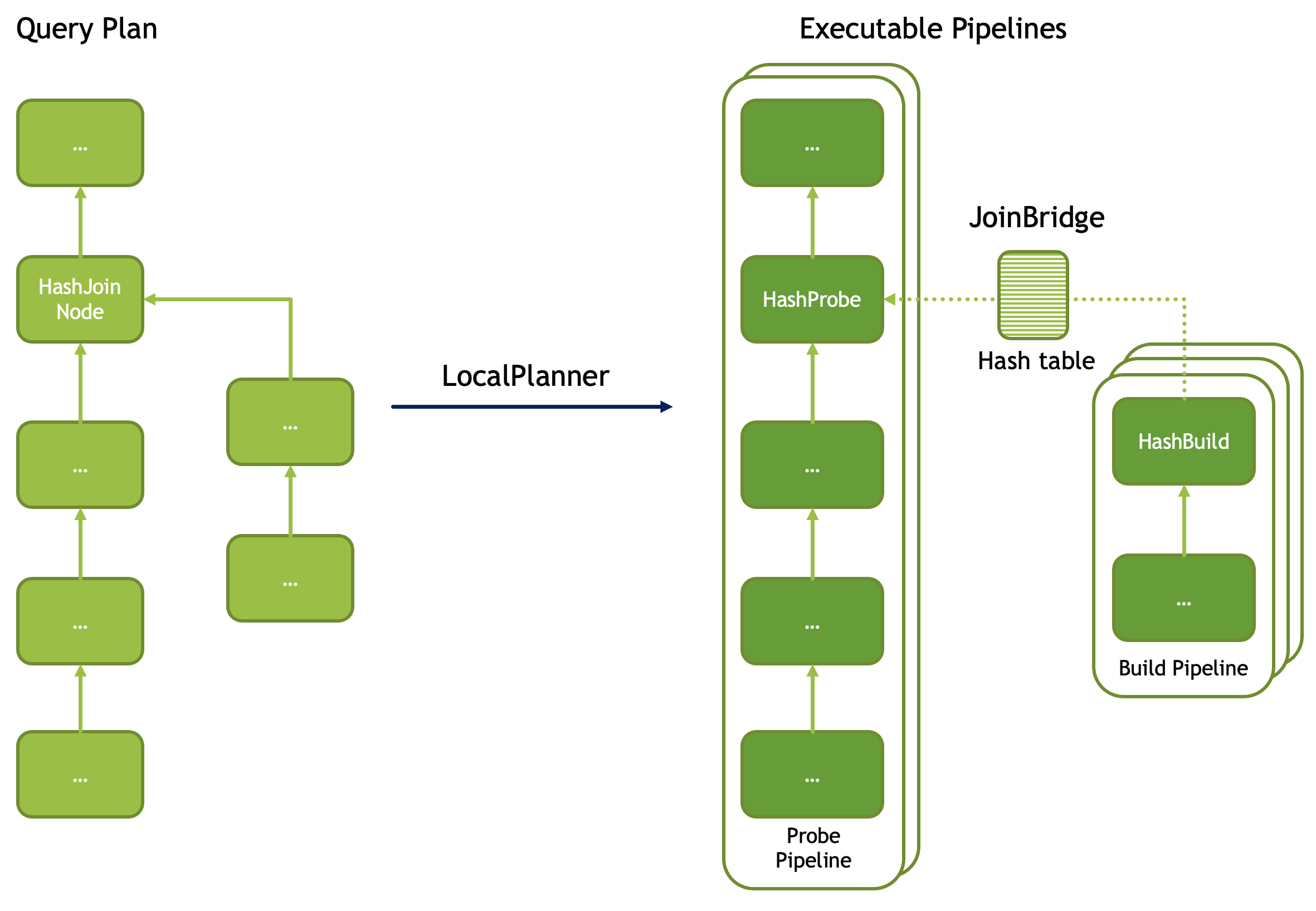
Join

A query plan with a join includes a HashJoinNode. Such a plan is translated into two pipelines: build and probe. Build pipeline is processing input from the build side of the join and uses HashBuild operator to build a hash table. Probe pipeline is processing input from the probe side of the join, probes the hash table and produces rows that match join criteria. Build pipeline provides the hash table to the probe pipeline via a special mechanism called JoinBridge. JoinBridge is like a future, where HashBuild operator completes the future with a HashTable as a result and HashProbe operator receives the HashTable when future completes.

Each pipeline can run with different levels of parallelism. In the example below, the probe pipeline runs on 2 threads, while the build pipeline runs on 3 threads. When the build pipeline runs multi-threaded, each pipeline processes a portion of the build-side input. The last pipeline to finish processing is responsible for combining the hash tables from the other pipelines and publishing the final table to the JoinBridge. When the probe pipeline for the right outer join runs multi-threaded, the last pipeline to finish processing is responsible for emitting rows from the build side that didn’t match the join condition.

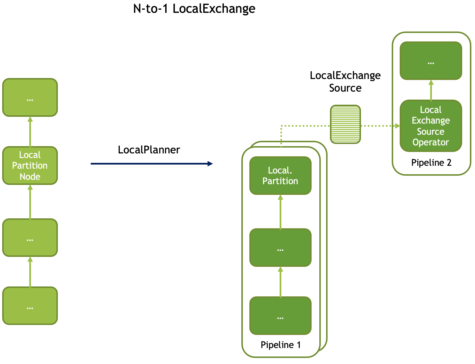
Local Exchange

A local exchange operation has multiple uses. It is used to change the parallelism of the data processing from multi-threaded to single-threaded or vice versa. For example, local exchange can be used in a sort operation where partial sort runs multi-threaded and then results are merged on a single thread. Local exchange operation is also used to combine results of multiple pipelines. For example to combine multiple inputs of the UNION or UNION ALL.

Here are some examples.

N-to-1 local exchange that could be used for combining partially sorted results for final merge sort.

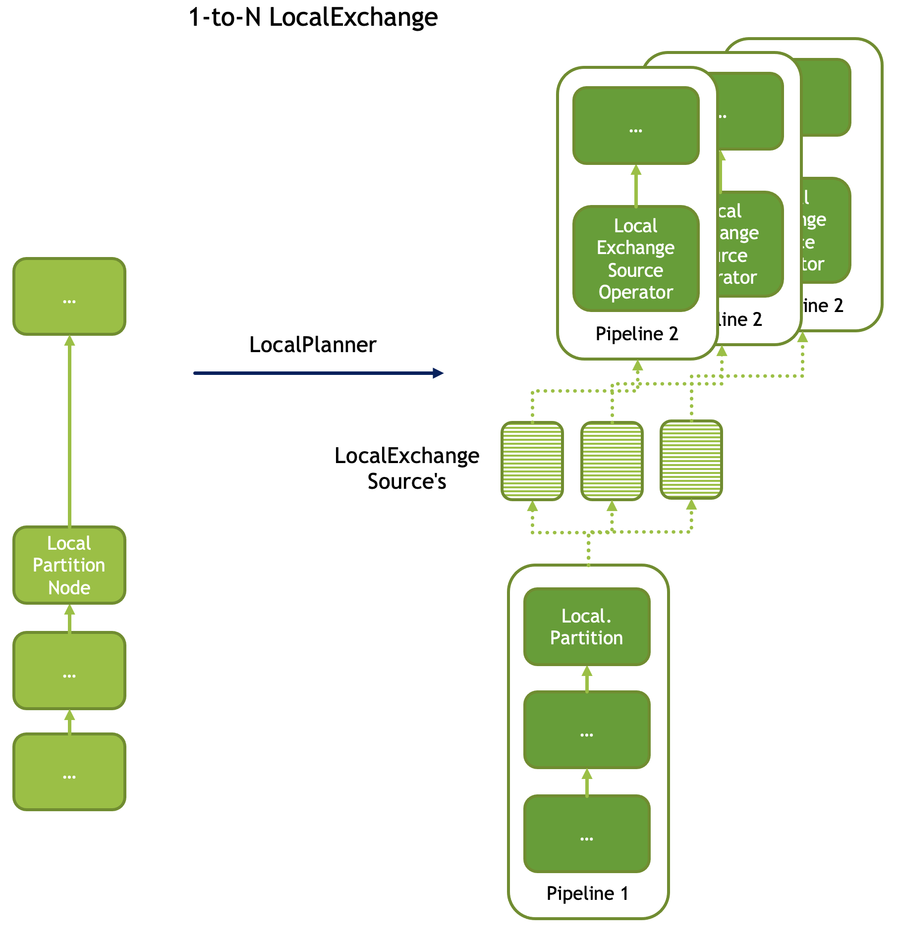
1-to-N local exchange to increase parallelism after an operation that must run single-threaded.

Local exchange used to combine data from multiple pipelines, e.g. for UNION ALL.