Understanding p-value and the confidence intervals in GeoLift

If you reached this section, it likely means that you were able to successfully run the previous steps in the guide and are now keen to deep-dive in understanding the details of the GeoLift package. In this part, we are going to explain the two methods employed by GeoLift to estimate the confidence interval and p-values of the Average Treatment Effect on the Treated (ATT). We will use the example from the Walkthrough to demonstrate and give some intuition how the method works.

From the Walkthrough example, we conducted a localized experiment in two locations (Chicago and Portland) for a period of 15 days. By using the GeoLift package, we were able to easily estimate the ATT of our marketing efforts on the two regions:

library(GeoLift)
library(ggplot2)
data(GeoLift_Test)

treated_locations = c("chicago", "portland")
post_period_start <- 91
post_period_ends <- 105

GeoTestData_Test <- GeoDataRead(
  data = GeoLift_Test,
  date_id = "date",
  location_id = "location",
  Y_id = "Y",
  X = c(), # empty list as we have no covariates
  format = "yyyy-mm-dd",
  summary = TRUE
)
#> ##################################
#> #####       Summary       #####
#> ##################################
#> 
#> * Raw Number of Locations: 40
#> * Time Periods: 105
#> * Final Number of Locations (Complete): 40

GeoTest <- GeoLift(
  Y_id = "Y",
  data = GeoTestData_Test,
  locations = c("chicago", "portland"),
  treatment_start_time = post_period_start,
  treatment_end_time = post_period_ends,
  ConfidenceIntervals = TRUE
)
#> Conformal method of Confidence Interval calculation unsuccessful. Changing Confidence Interval calculation method to jackknife+.
GeoTest
#> 
#> GeoLift Output
#> 
#> Test results for 15 treatment periods, from time-stamp 91 to 105 for test markets:
#> 1 CHICAGO
#> 2 PORTLAND
#> ##################################
#> #####     Test Statistics    #####
#> ##################################
#> 
#> Percent Lift: 5.4%
#> 
#> Incremental Y: 4667
#> 
#> 90% Confidence Interval: (-2450.734, 11349.93)
#> 
#> Average Estimated Treatment Effect (ATT): 155.556
#> 
#> The results are significant at a 95% level. (TWO-SIDED LIFT TEST)
#> 
#> There is a 1.2% chance of observing an effect this large or larger assuming treatment effect is zero.

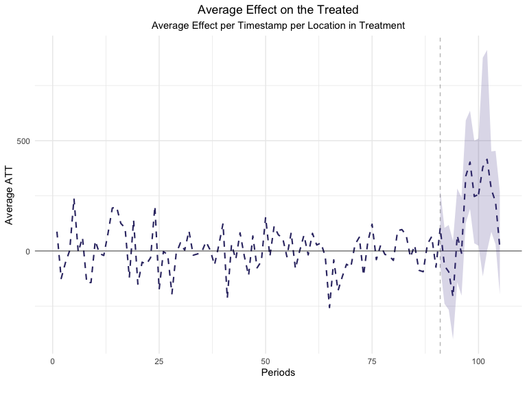
We can also visualize the ATT per day using the plot function

plot(GeoTest, type = "ATT")
#> You can include dates in your chart if you supply the end date of the treatment. Just specify the treatment_end_date parameter.

PlotLiftBest

But how did GeoLift estimate these confidence intervals and p-values?

Default: Conformal Inference Method

As the default, GeoLift - or more accurately the Augmented Synthetic Control package - uses a method called Conformal Inference to estimate the confidence interval for the ATT. This method developed in 2022 by researchers Victor Chernozhukov, Kaspar Wütrich, and Yinchu Zhu has been shown to work with multiples approaches for estimating counterfactual outcomes, such as Synthetic Control (the case here), Difference-in-Differences, factor and matrix completion models, among others. It demonstrates high small-sample performance or when there are (reasonable) misspecifications of the model.

Estimating the p-value

From the paper, the p-value (i.e. the probability of observing a data as or more absurd, assuming that the null-hypothesis is true) for a chosen date is given by

Equation 1

where

Equation 2

and is the residual (i.e. the error) between what an Augmented Synthetic Control Model (hereafter referred simply as ‘model’) estimated and what was observed on the chose date for the treated location (if there are more than 1 treated location, they are grouped and averaged). The function defines the test statistics, and it can be interpreted as an error functions, such as Mean Squared Error and Mean Absolute Error:

Equation 3

where is the number of ‘dates’ in the Post-Treatment Period, is the number of dates date in the Pre-Treatment Period, and indicates the last date available for the analysis (so ).

Coming back to the first equation, stands for a block permutation, which is a one-to-one mapping that reorder the dates (from both Post-Treatment and Pre-Treatment Periods). One example of a block permutation is “shifting all dates forward by 1*“, so that in the simplest example the original data would look like this:

data.frame(values = c(40, 10, 20, 30), dates = c(1, 2, 3, 4))
#>   values dates
#> 1     40     1
#> 2     10     2
#> 3     20     3
#> 4     30     4

and after our block permutation they become:

data.frame(values = c(40, 10, 20, 30), dates = c(4, 1, 2, 3))
#>   values dates
#> 1     40     4
#> 2     10     1
#> 3     20     2
#> 4     30     3

The case above is an example of overlapping moving block permutations , for the case where , and is the default block permutation from the Augmented Synthetic Control package to calculate point wise confidence intervals. The elements of are indexed by and a permutation is defined as

Equation 4

So reading back the equation and using overlapping moving block permutations for , we can translate the equation as “The probability that the residual was caused just by noise is the share of dates where we had an error smaller than . where refers to a Day of Interest (DoI) in the Post-Treatment Period, and the dates included for the analysis are all dates in the Pre-Treatment Period and the DoI itself.

Estimating the Confidence Interval

The confidence interval is estimated by repeating the estimation of the p-value for a range of G values by subtracting from the observed value of the treated unit at the DoI. The reason why we subtract a value , can be thought of as ‘removing the real effect that the treatment caused’, so that when we remove the treatment effect perfectly, our algorithm above should indicate a high p-value.

Let’s take the scenario where we have our target value in the Pre-Treatment Period following a normal distribution of expected value (1.0) and standard deviation 0.1. With the treatment, the expected value of the target increased by 30% while keeping the same standard deviation:

  days <- 100
  post_treament_start_day <- 70
  expected_values <- rep(1.0, days)
  expected_values[post_treament_start_day:days] <- expected_values[post_treament_start_day:days] * 1.3
  observed_values <- rnorm(days, expected_values, 0.1)
  dummy_data <- data.frame(date = seq(days), Y = observed_values)
  ggplot(dummy_data, aes(x = date, y = Y)) + 
    geom_line(color = 'skyblue3') + 
    geom_vline(aes(xintercept = post_treament_start_day), linetype='dashed', color = 'gray20') +
    scale_y_continuous(limits = c(0, 2))

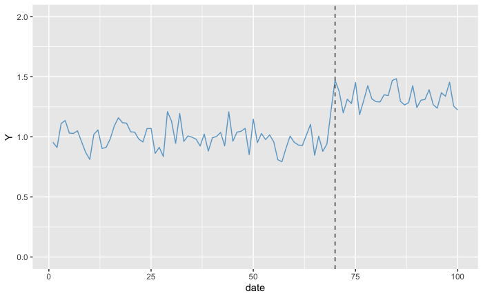
Which means that for the null-hypothesis “the probability of observing a data as or more absurd, assuming that there is no increase”, we expect to obtain a quite low p-value. After all, we can clearly see the different level that Y is in the Post-Treatment Period. But what if we wanted to estimate the p-value not for no increase but for an increase of 20%? In this case, we subtract 0.2 from all the values in the Post-Treatment Period from the treated units:

  altered_dummy_data <- dummy_data
  h0 <- 0.2
  altered_dummy_data$Y[post_treament_start_day:days] <- altered_dummy_data$Y[post_treament_start_day:days] - h0
  ggplot(altered_dummy_data, aes(x = date, y = Y)) + 
    geom_line(color = 'skyblue3') + 
    geom_vline(aes(xintercept = post_treament_start_day), linetype='dashed', color = 'gray20') +
    scale_y_continuous(limits = c(0, 2))

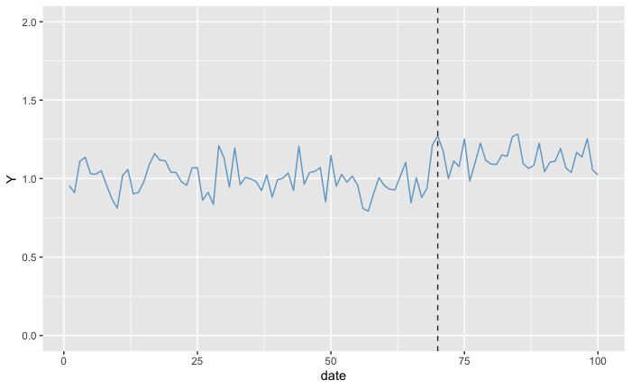
As we can see with the plots, the target values at the Post-Treatment Period are much closer to the values in the Pre-Treatment Period. As a consequence, we expect the p-value to be much higher than before, but still (from looking only at the plot) the p-value should be below 0.5 as it looks that most often the values in the Post-Treatment are above the values in the Pre-Treatment Period.

Now what would happen if we removed exactly the actual increase we got from the treatment?

  altered_dummy_data <- dummy_data
  h0 <- 0.3
  altered_dummy_data$Y[post_treament_start_day:days] <- altered_dummy_data$Y[post_treament_start_day:days] - h0
  ggplot(altered_dummy_data, aes(x = date, y = Y)) + 
    geom_line(color = 'skyblue3') + 
    geom_vline(aes(xintercept = post_treament_start_day), linetype='dashed', color = 'gray20') +
    scale_y_continuous(limits = c(0, 2))

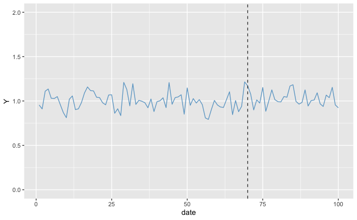
We don’t see any difference between before and after the treatment, so the p-value should be quite high. So by applying a shift to the target values at the treatment locations at the Post-Treatment Period, we are assessing the likelihood of each one of the shifts. After we execute this process several times, we obtain the p-values for each one of the possible treatment effects considered, resulting in something that looks and works similar (It is not!) to a probability density function of the treatment effect.

Implementation of the algorithm

The Conformal Inference method proposed by the authors and used by GeoLift mainly consists of the following steps for each day in the post-treatment period (Algorithm 1 from the paper):

Subtract to all treated locations in the Day of interest (DoI), which is in the Post-Treatment Period, a constant H0.
State the DoI that is originally in the Post-Treatment Period to be in the Pre-Treatment Period
Train a new Augmented Synthetic Control Model (though it could be any Synthetic Control, Difference-in-Differences, or Factor/Matrix Completion model) based on the new data. I.E. on a data where the DoI is considered to be in the Pre-Treatment Period for all locations
Collect the residuals (i.e. the error / the ATT) between what the new model predicted
Apply a ‘cost’ function to the residual of each day (e.g. abs(resi))
Observe for which % of days in the Pre-Treatment Period (again, which includes DoI) the model had a higher ‘cost’ than on the DoI. This gives you an estimate of the ‘p-value’ for the DoI and step size H0: “The probability of observing a data as absurd or more than this, assuming that the effect is H0”
Repeat steps 1 ~ 6 for a range of values H0 to obtain the ‘p-value’ for each magnitude
To find the limits of a confidence interval of size (1 - alpha), select the lowest/greatest value H0 where the p-value was greater or equal to alpha to obtain the lower/upper bound

We demonstrate below how to implement the method and show that the output is aligned with what GeoLift does for the first day of the Post-Treatment Period (i.e. day 91):

library(augsynth)
day_of_interest <- 91
h0 <- 0
cost_funct = function(residuals) return (abs(residuals))

# We create a copy of the original data we can alter without worries
new_geo_data <- GeoTestData_Test

# 1) Subtract to all treated locations in the Day of interest (DoI) a constant H0
new_geo_data$Y[(new_geo_data$time == day_of_interest) & (new_geo_data$location %in% treated_locations)] <- new_geo_data$Y[(new_geo_data$time == day_of_interest) & (new_geo_data$location %in% treated_locations)] - h0

# 2) State the DoI that is originally in the Post-Treatment Period to be in the Pre-Treatment Period
pretreatment_period <- c(1:(post_period_start - 1), day_of_interest) # define which days are in the Pre-Treatment Period
is_pretreatment_period <- GeoTestData_Test$time %in% pretreatment_period
is_treated_unit <- (!is_pretreatment_period & GeoTestData_Test$location %in% treated_locations)
new_geo_data$D <- as.integer(is_treated_unit)


# 3) Train a new Augmented Synthetic Control Model (though it could be any Synthetic Control, Difference-in-Differences, or Factor/Matrix Completion model) based on the new data. I.E. on a data
synthetic_control_model <- augsynth::augsynth(
    form = as.formula("Y ~ D"),
    unit = location,
    time = time,
    data = new_geo_data,
    t_int = post_period_start + 1, # +1 because we sent the DoI to the pre-treatment period
    progfunc = "none",
    scm = TRUE,
    fixedeff = TRUE,
)
#> One outcome and one treatment time found. Running single_augsynth.


# 4) Collect the residuals (i.e. the error / the ATT) between what the new model predicted.
residuals <- predict(synthetic_control_model, att = T)[1:post_period_start] # here we already select that we will use only from the Pre-Treament Period

# 5) Apply a 'cost' function to the residual of each day (e.g. abs(resi))
costs <- cost_funct(residuals)

# 6) Observe for which % of days in the Pre-Treatment Period (again, which includes DoI) the model had a higher 'cost' than on the DoI. This gives you an estimate of the 'p-value' for the DoI and step size H0: "The probability of observing a data as absurd or more than this, assuming that the effect is H0"
p_value <- mean(costs[day_of_interest] <= costs) 

# Observe that the result is exactly what was in the output of GeoLift
print(p_value)
#> [1] 0.2857143
print(GeoTest$summary$att[day_of_interest, ])
#>    Time Estimate lower_bound upper_bound     p_val
#> 91   91 108.8099   -82.98491    300.6048 0.2857143

As you can see, the p-value we obtain matches perfectly with what GeoLift shows. We obtain the confidence interval by repeating the previous step for a range of values of H0, and collecting the p-value associated to each H0 value:

# 7) Repeat steps 1 ~ 6 for a range of values H0 to obtain the 'p-value' for each magnitude
# Let's then put the previous code in a function
get_p_value = function(h0){
  new_geo_data <- GeoTestData_Test
  pretreatment_period <- c(1:(post_period_start - 1), day_of_interest)
  is_pretreatment_period <- GeoTestData_Test$time %in% pretreatment_period
  is_treated_unit <- (!is_pretreatment_period & GeoTestData_Test$location %in% treated_locations)
  new_geo_data$D <- as.integer(is_treated_unit)
  
  # the only change: we subtract the related impact from the observed values
  new_geo_data$Y[(new_geo_data$time == day_of_interest) & (GeoTestData_Test$location %in% treated_locations)] <- new_geo_data$Y[(new_geo_data$time == day_of_interest) & (GeoTestData_Test$location %in% treated_locations)] - h0
  
  synthetic_control_model <- suppressMessages(
      augsynth::augsynth(
      form = as.formula("Y ~ D"),
      unit = location,
      time = time,
      data = new_geo_data,
      t_int = post_period_start + 1,
      progfunc = "none",
      scm = TRUE,
      fixedeff = TRUE,
    )
  )
  
  residuals <- abs(predict(synthetic_control_model, att = T)[1:post_period_start])
  reference_residual <- abs(residuals[post_period_start])
  p_value <- mean(reference_residual <= abs(residuals))
  
  return(p_value)
  
}

# As we got for day 91 an estimated ATT of 108.810 let's try  a wide range of values from there.
# Let's try a wide range of values based on the expected ATT for the DoI. We are going to use 6 standard deviations which would be more than enough if the distribution were normal
# We use the same parameters as the default of GeoLift for comparability
grid_size = 250
sd = sqrt(mean(GeoTest$ATT[post_period_start:post_period_ends]**2))
grid <- seq(GeoTest$ATT[day_of_interest][[1]] - 6*sd, GeoTest$ATT[day_of_interest][[1]] + 6*sd,  length.out = grid_size)

# We calculate the p-value for each one of the defined H0
p_values <- sapply(grid, get_p_value)

# 8) To find the limits of a confidence interval of size (1 - alpha), select the lowest/greatest value H0 where the p-value was greater or equal to alpha to obtain the lower/upper bound
# Let's suppose we want the 90% confidence interval:
alpha = (1 - 0.9)
lower_bound <- min(grid[p_values >= alpha])
upper_bound <- max(grid[p_values >= alpha])
print(lower_bound)
#> [1] -75.93094
print(upper_bound)
#> [1] 293.5508

# which again, will be similar to what GeoLift stated:
print(GeoTest$summary$att[day_of_interest, ])
#>    Time Estimate lower_bound upper_bound     p_val
#> 91   91 108.8099   -82.98491    300.6048 0.2857143

As you can see the values we got are almost exactly the ones provided by GeoLift, with the difference originating from the grid of tested values being different.

The backfall: Jackknife Method

While Conformal Inference is proven to be robust in many scenarios, it is not guaranteed to work everytime. Most commonly, Conformal Inference can fail when

there is not enough days in the Pre-Treatment Period
the true impact (called in the paper as Shock Sequence Ut) is not stationary or not weakly dependent
the data is not stationary and not weakly dependent when our model is misspecified or inconsistent

When Conformal Inference fails, GeoLift falls back to the second method called ‘jackknife+’, which works similar to Conformal Inference in the aspect that we alter what constitutes the Pre-Treatment Period. In Jackknife+, for each day in the Pre-Treatment Period

We remove it from the Pre-Treatment Period and put it on the Post-Treatment Period
We train another Augmented Synthetic Control Model
We calculate the absolute difference (abs(e)) between what was observed in and what the model estimated
For each day in the original Post-Treatment Period, we collect the difference between what was observed and what the model predicted. From this vector we create 2 others, one where we add abs(e) and one where we subtract abs(e) creating respectively the upper and lower bound for this iteration
We store these lower and upper bound values
The confidence interval is then obtained by getting the respective quantiles from the upper/lower bound

As before, below is a demonstration on how Jackknife works:

train_augmented_synthetic_control = function(geo_data, treatment_start_date){
  
  new_geo_data <- geo_data
  pretreatment_period <- 1:treatment_start_date
  is_pretreatment_period <- new_geo_data$time %in% pretreatment_period
  is_treated_unit <- (!is_pretreatment_period & new_geo_data$location %in% treated_locations)
  new_geo_data$D <- as.integer(is_treated_unit)
  
  # 2) We train another Augmented Synthetic Control Model 
  model <- suppressMessages(
    augsynth::augsynth(
      form = as.formula("Y ~ D"),
      unit = location,
      time = time,
      data = new_geo_data,
      t_int = treatment_start_date, # since we removed the date from the Pre-Treatment Period and put it in the Post-Treatment Period
      progfunc = "none",
      scm = TRUE,
      fixedeff = TRUE,
    )
  )
  return (model)
}


jacknife_estimator = function(geo_data, treatment_start_date, treatment_end_date, iteration_day){
  # Make a copy of original data
  new_geo_data <- geo_data
  post_treatment_days <- treatment_start_date:treatment_end_date
  
  # 1) We remove it from the Pre-Treatment Period and put it on the Post-Treatment Period
  # Define what is in the Pre- and Post-Treatment Periods
  # if it is the iteration_day, then we state that it is the the Post-Treatment period but putting it right before the original start and shift all following days in the original Pre-Treatment period 'left'
  new_geo_data$time = sapply(
    new_geo_data$time, function(x) ifelse(
      x == iteration_day, treatment_start_date - 1, 
      ifelse((x < treatment_start_date) & (x > iteration_day), x - 1, x)
      )
    )
  
  # 2) We train another Augmented Synthetic Control Model 
  synthetic_control_model <- train_augmented_synthetic_control(new_geo_data, treatment_start_date - 1)

  # 3) We calculate the absolute difference (abs(e) )between what was observed in D_pre and what the model estimated
  residuals <- predict(synthetic_control_model, att = F)
  error <- abs(mean(new_geo_data$Y[(new_geo_data$time == (treatment_start_date - 1)) & (new_geo_data$location %in% treated_locations)]) -  residuals[treatment_start_date - 1])
  
  # 4) For each day in the original Post-Treatment Period, we collect the difference between what was observed and what the model predicted. From this vector we create 2 others, one where we add abs(e) and one where we subtract abs(e) creating respectively the upper and lower bound for the counterfactual
  upper_bound <- c(residuals[post_treatment_days], mean(residuals[post_treatment_days]))  +  error
  lower_bound <- c(residuals[post_treatment_days], mean(residuals[post_treatment_days])) - error
  
  # 5) We store these lower and upper bound values   
  return(list(upper_bound = upper_bound, lower_bound = lower_bound, error = error))
}


augsynth_model <- train_augmented_synthetic_control(GeoTestData_Test, post_period_start)
obs_values <- (predict(augsynth_model, att = T) + predict(augsynth_model, att = F))[post_period_start:post_period_ends]
obs_values <- c(obs_values, mean(obs_values))

upper_bound = c()
lower_bound = c()
# ... for each day D_pre in the Pre-Treatment Period (we run the previously defined steps)
for (day in 1:(post_period_start - 1)){
  result <- jacknife_estimator(GeoTestData_Test, post_period_start, post_period_ends, day)
  upper_bound <- rbind(upper_bound, result$upper_bound)
  lower_bound <- rbind(lower_bound, result$lower_bound)
}

# 6) The confidence interval is then obtained by getting the respective quantiles from the upper/lower bound
# using the same parameters as before:
alpha = (1 - 0.9) # for 90% confidence interval

# We obtain the confidence intervals for the ATT by subtracting from what was observed (factual) the upper/lower bounds of the counterfactual
post_treament_upper_bound <- obs_values - apply(lower_bound, 2, function(x) quantile(x, alpha/2))
post_treament_lower_bound <- obs_values - apply(upper_bound, 2, function(x) quantile(x, 1 - alpha/2))

print(post_treament_upper_bound)
#>         91         92         93         94         95         96         97 
#> 331.336571 155.656817 125.461659   4.687216 286.346779 216.483095 567.128420 
#>         98         99        100        101        102        103        104 
#> 630.101980 471.727499 479.616984 588.369348 636.523734 505.765583 443.125831 
#>        105            
#> 235.131135 378.330998
print(post_treament_lower_bound)
#>         91         92         93         94         95         96         97 
#> -126.25015 -301.95956 -329.52402 -452.65056 -171.83181 -238.57023  113.75990 
#>         98         99        100        101        102        103        104 
#>  177.19184   16.16962   16.43517  120.48222  175.10239   48.46091  -11.15596 
#>        105            
#> -220.89674  -81.69113

The last value on the vectors ‘post_treament_upper_bound’ and ‘post_treament_lower_bound’ refer to the upper and lower bound of the ATT for the whole Post-Treatment Period. If we multiply them by the number of locations (2) and the number of days in the Post-Treatment Period, we obtain the interval provided by GeoLift:

GeoTest
#> 
#> GeoLift Output
#> 
#> Test results for 15 treatment periods, from time-stamp 91 to 105 for test markets:
#> 1 CHICAGO
#> 2 PORTLAND
#> ##################################
#> #####     Test Statistics    #####
#> ##################################
#> 
#> Percent Lift: 5.4%
#> 
#> Incremental Y: 4667
#> 
#> 90% Confidence Interval: (-2450.734, 11349.93)
#> 
#> Average Estimated Treatment Effect (ATT): 155.556
#> 
#> The results are significant at a 95% level. (TWO-SIDED LIFT TEST)
#> 
#> There is a 1.2% chance of observing an effect this large or larger assuming treatment effect is zero.
print(tail(post_treament_upper_bound, 1) * length(treated_locations) * (post_period_ends - post_period_start + 1))
#>          
#> 11349.93
print(tail(post_treament_lower_bound, 1) * length(treated_locations) * (post_period_ends - post_period_start + 1))
#>           
#> -2450.734

Thus Jackknife+ method provides an estimate of the Confidence Interval for the ATT that is based on the error that model has on each day of the Pre-Treatment Period if it was put in the Post-Treatment Period. Because the days that got moved actually didn’t receive the treatment, the error that the model has on each one of these days gives some insight on the accuracy of our model in estimating the counter-factual for the treated locations during the Post-Treatment Period. Because we remove one day at a time, the coefficients found for our model aren’t too different to what we obtain using the whole Pre-Treatment Period data. However, because we use the absolute value of the error of the model in each one of the moved dates, the confidence interval estimated by this method tends to be larger than the true confidence interval of the estimated treatment effect.

Frequently Asked Questions

The estimation of the Confidence Intervals are supposed to be deterministic from the documentation, but when I run it it varies.

The estimation of the Confidence Intervals and the p-value using Conformal Inference is indeed deterministic when using overlapping moving block permutations. If instead we were to consider all block permutations (or sample from them) which happens when the parameter conformal_type is "iid", then GeoLift extract ns samples from all the possible block permutations, which means that the estimated confidence intervals and the p-value can vary slightly

When I ask GeoLift to provide confidence intervals for the ATT it raises a warning saying that the Conformal Inference method failed. Why does this happen?

This happens because when trying to estimate the p-values for the different possible lifts, all the p-values estimated were too low. As a consequence of all p-values being too small, when we execute step (8) lower_bound <- min(grid[p_values >= alpha]), we can’t find any case where a p-value was greater than the alpha we require for the confidence interval (remember that alpha = 1 - confidence interval size). This happens if one or more conditions for the Conformal Inference method are not satisfied, with one of the most common being that the observations on each day are not ‘iid’, which is usually solved by changing the conformal_type input to "block".

There are cases where the ATT for the Post-Treatment Period indicates for a 90% confidence interval a lower bound below 0, even though the p-value is low (e.g. 5%). Why does this happen?

This often happens because either

You used different conformal_type for the p-value and for the confidence interval,
you used Jackknife+ for one of the metrics and Conformal Inference for the other. This usually happens when Conformal Inference method fails to estimate the confidence interval and fallbacks to the Jackknife+, or
the estimation of the p-value using the Conformal Inference method is inaccurate for the specific case you are using (see step (7) in the Conformal Inference explanation above).

For the last point, you can verify that is the source of the problem by plotting the estimated p-values for each assumed lift (given by the variable grid on step (7)). When you plot(grid, p_values), you should see a curve resembling a normal distribution. It doesn’t have to be normal, as it can be asymmetric and long-tailed, but it shouldn’t deviate much from what a normal distribution looks like. Cases that don’t look like a normal distribution is when the curve is bi-modal or the p-value for points close to each other in the grid to are much different.

Should I expect the confidence intervals estimated by the Jackknife+ and Conformal Inference to be the same?

They should be similar, though Jackknife+ should indicate a wider interval than Conformal Inference. The cause originates in step (4) of the Jackknife algorithm described above, where we add/subtract the absolute error to estimate the upper/lower bound in one iteration.

Default: Conformal Inference Method​

Estimating the p-value​

Estimating the Confidence Interval​

Implementation of the algorithm​

The backfall: Jackknife Method​

Default: Conformal Inference Method

Estimating the p-value

Estimating the Confidence Interval

Implementation of the algorithm

The backfall: Jackknife Method