TL;DR​

• This blog post demonstrates how to deal with treated observations in sequential GeoLift testing.
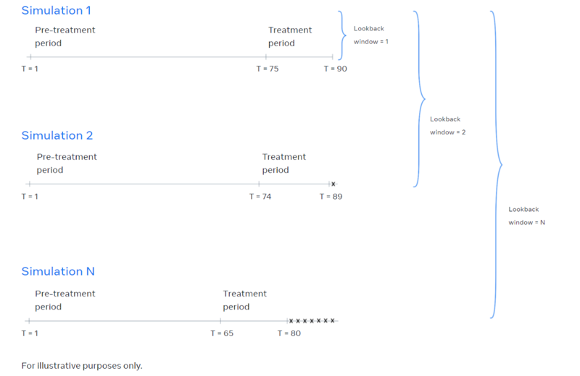
• Currently, when running two sequential GeoLifts, the treatment period of the first experiment becomes part of the pre-treatment period of the second experiment, potentially affecting results and power calculations.
• To prevent this, you can replace the treatment locations in the first experiment with the best counterfactual available. Once the treatment location has been replaced, make sure to expand the control donor pool with said series.
• We introduce our ReplaceTreatmentSplit function to replace the treated location units, easily implementing our proposed solution.

Introduction​

Advertisers have many questions to answer like, “What’s the incremental impact of this media channel?” and “What’s the budget elasticity of my investment in this channel?”. These questions and more can be answered using GeoLift.

Since each question is different and we cannot answer them all at the same time, we need to decide which of them we should answer first by building a learning agenda. Our agenda holds everything from business questions and hypotheses to specific experiment designs that will give us the answers we are looking for. For the sake of simplicity, imagine we have two business questions, and we run our first GeoLift (experiment 1) to answer the first one and would like to design a new GeoLift (experiment 2) to give an answer to our second inquiry.

However, running a second GeoLift immediately after the previous one is not that simple.

Sequential GeoLift testing​

At a first glance, we have a couple of options:

Option 1: Repeating our experiment 1 treatment group in experiment 2, excluding the experiment 1 periods.​

This implies that we will remove experiment 1 time periods from the pre-treatment period, meaning we will get the same time series we had before experiment 1 was run. Furthermore, if we rerun the power analysis with this series, we will get the same treatment group we had for experiment 1.

While an attractive option, it lacks flexibility due to the fact that we will probably choose the same treatment we did before experiment 1. Furthermore, we should make sure that the GeoLift model is able to accurately predict the most recent time-stamps, using the latest market dynamics. For example, if we had a test for all of December, then the model trained up to November might struggle to predict January due to different spending trends. Moreover, if the treatment was very long, this might make it very hard to justify tying the set of pre-treatment periods for experiment 1 to the periods during experiment 2.

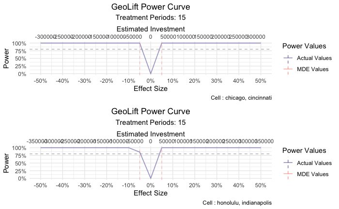
Option 2: Rerunning the power analysis for experiment 2, without excluding experiment 1 periods.​

Without removing the periods from experiment 1, we will preserve the autocorrelation within the time series and avoid the sudden change that may occur, while keeping the latest time-stamps. Having said this, going with this option poses another threat. Locations that were used as a treatment group in experiment 1 will probably not be chosen as a good setup in the GeoLift ranking algorithm. When we run simulations using those locations, the simulated effect will probably be far off from the observed effect, since they already had a previous treatment that we are not considering.

If the locations selected as the treatment group presented a good setup for experiment 1, then at least some of them should be selected to be part of the treatment of experiment 2.

Our solution: Replace treatment group values from experiment 1​

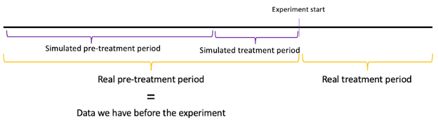
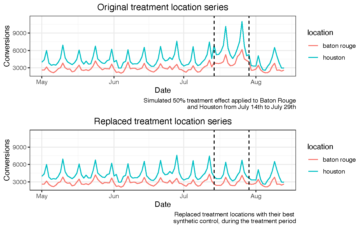
Our goal is maximizing the amount of data we have without excluding any periods and guaranteeing that our dataset does not contain any structural changes (treatment applied to certain locations in experiment 1). To do so, we recommend replacing the values of the locations that were treated during experiment 1, during the periods in which the treatment occurred and including them in the control donor pool. For reference, here’s a picture of what this looks like.

Here’s an example of our pseudo-code:

1. Define locations that were treated and treatment period during experiment 1.
2. Fit a GeoLift counterfactual to each of the treatment locations, training it on experiment 1’s pre-treatment period.
3. Only keep the counterfactual that has the closest match to a treatment location in the pre-treatment period (using absolute L2 imbalance, A.K.A. the sum of squared differences between treatment and control prior to the experiment).
4. Replace the selected treatment location by its counterfactual values during the experiment 1’s treatment period.
5. Reassign the replaced treatment location to the control donor pool.
6. Repeat this process until there are no more treatment locations left.

This solution has three clear benefits:

• We preserve the time series structure without excluding any data.
• We replace the structural change in the treatment locations by our best estimate of what would have happened if they had not been treated.
• We have a higher chance of providing better counterfactual fits for the replaced treatments because we are enlarging the control donor pool with each replacement.

Data-driven validation​

The last of these benefits does not necessarily mean that we will always be better off. Particularly, the algorithm will provide the same L2 imbalance values for cases where we have a smaller treatment size given that the added value of the replaced treatment to the control donor pool will not be as large.

In order to understand what was the average impact that our algorithm had on L2 imbalance, we decided to run a random selection of locations to build different treatment groups of 5 locations. We then passed those random groups through the algorithm, and compared it to the L2 imbalance that the counterfactual would have if the replaced treatment had not been added to the control donor pool. That is what we call the L2 imbalance improvement ratio:

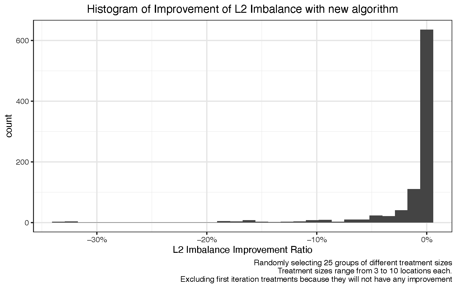
While the majority of the observations for the L2 imbalance improvement ratio are close to zero, there is a negative long tail that shows that there are some cases where our algorithm works better than the alternative.

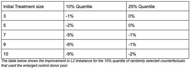
To make our finding more robust, we repeated the simulations with randomly selected treatment groups of different sizes. Looking at the 10% and 25% quantiles of the histogram provided above for each treatment size, we saw improvements in L2 imbalance of up to 8% in the 10% quantile. Naturally, the larger the treatment group, the higher the benefit of our proposed solution, in line with our aforementioned hypothesis.

How to implement the algorithm?​

We have recently landed a simple method for you to use if you would like to leverage this algorithm. Simply implement the ReplaceTreatmentSplit function, specifying what the treatment locations and the treatment start date and end date for experiment 1 are. You can pick up the replaced dataset from the $data argument in the list. The $l2_imbalance_df will give you the data frame of L2 imbalances for each treatment location when they were replaced.

# Import libraries and transform data.
library(GeoLift)
data(GeoLift_Test)
geo_data <- GeoDataRead(data = GeoLift_Test,
                        date_id = "date",
                        location_id = "location",
                        Y_id = "Y",
                        X = c(), #empty list as we have no covariates
                        format = "yyyy-mm-dd",
                        summary = TRUE)
treatment_group <- c(‘chicago’, ‘portland’)

# Replace treatment locations for best counterfactual.
g <- ReplaceTreatmentSplit(
  treatment_locations = treatment_group,
  data = geo_data,
  treatment_start_time = 90,
  treatment_end_time = 105,
  model = "none",
  verbose = TRUE
)

# Extract replaced data.
new_geo_data <- g$data

What’s up next?​

Keep your eye out for our coming blog posts, around topics like:

• When should I use Fixed Effects to get a higher signal to noise ratio?
• Long term branding measurement with GeoLift.

TL;DR​

• The success of a geo-based experiment greatly depends on the Market Selection process.
• In the GeoLift package, we use historical data and a simulation-based approach to identify the best set of treatment and control locations based on the constraints specified by the user.
• Selecting an appropriate value for the lookback_window parameter (the amount of pre-treatment periods that will be considered) is a very important part of the process.
• Based on the analysis presented in this note, we generally recommend using 1/10th of the pre-treatment period as a simulation lookback_window (especially if your time-series has a lot of variability across time).

What is considered a simulation in GeoLift?​

Essentially, before running the actual test, we are running a series of geo experiments to determine which is the best setup that will pave the way to success. As explained in further detail in our Blueprint Course, the GeoLift Market Selection process simulates a large number of geo experiments to determine which is the best test and control setup for you.

In each simulation a treatment effect is applied over a treatment group during the treatment period. Then, GeoLift then trains a counterfactual for the treatment group by using all of the pre-treatment periods prior to the experiment to assess the model's performance. Let’s breakdown each of these five components:

• The treatment effect: is the Lift percentage that will be applied to a set of locations during the testing period.
• The treatment group: these are a set of locations that will be exposed to the treatment effect.
• The counterfactual: these are a set of locations that are used to estimate what would have happened to the treatment group if it had not been exposed to the treatment effect. An easy way to think about it is as a weighted average of all the locations that are not part of the treatment group.
• The treatment period: represents the moments in which the treatment group will be exposed to the treatment.
• The pre-treatment period: this refers to the amount of periods that will be used to build the counterfactual, where there was no simulated difference between locations. During this period, the counterfactual and the treatment group should have a similar behavior.

Applying different effects to the same group in the same period allows us to holistically determine what the Minimum Detectable Effect (MDE) for that setup will be. Among other metrics, this helps us understand whether we are dealing with a combination of locations that will have a higher likelihood of observing small effect sizes. However, seasonalities and variations throughout time make can difficult to estimate the MDE with complete certainty. Fortunately, we can reduce this uncertainty by taking a look at the past!

Introducing the lookback window parameter.​

Our first simulation uses the most recent/latest periods in our series as our treatment period and all of the remaining periods as our pre-treatment period. This gives us the metrics we need to rank treatment groups for those time periods.

As stated in our GeoLift Walkthrough, we can increase the number of simulated time periods by changing the lookback_window. The lookback_window indicates how far back in time the simulations for the power analysis will go. By increasing the lookback_window, we subtract the last period from the previous simulation’s total duration and repeat the process over the remaining periods. Finally, we calculate the average metrics for each treatment group over all of the runs in different periods.

For example, imagine we have a 90 day long series with different locations and we would like to simulate a 15 day test, with a 2 day lookback_window.

• In the first simulation, the treatment period is made up of the most recent dates and Lift is simulated on it. The remainder, the pre-treatment period, is used to build a counterfactual. So, with a test duration of 15 days, for this iteration we use periods 1 to 75 as a pre-treatment period and periods 76 to 90 as a treatment period.
• For our second simulation, the treatment period is shifted by one timestamp. We use periods 1 to 74 as a pre-treatment period and periods 75 to 89 as a treatment period.
• We then construct average metrics per each treatment group, using these two simulations. In essence, we are repeating this flow until the number of time periods shifted is equal to the lookback_window parameter.

In this context, more simulations allow us to have a more robust estimate of the metrics for each treatment group, observing if the same behavior occurs across different simulated treatment and pre-treatment periods. The intuitive idea here is that we would like to capture some of the variability in the time series in our test setups, to avoid assuming something that could be different in the future.

There’s a tradeoff: robustness vs preciseness​

The more we look back into the past, the more simulations per treatment group we will have. This will make our estimates more robust and allow us to make safer predictions with regard to the pre-test metrics.

However, the more we look back into the past, the less precise our simulation will be as compared to the actual result. Removing the last periods we have prior to the test leads to two major effects:

• Our simulations become less precise because they have a smaller amount of periods to build the counterfactual than what the actual experiment will have.
• The accuracy of our simulation will be reduced since we are shortening the time that is being considered by the algorithm’s pre-treatment period.

Given this tradeoff, we need to choose the amount of simulations we run considering the potential they have but keeping in mind that they also have a downside. Moreover, it is important to note that incresing the lookback_window parameter will exponentially increase the number of simulations performed in the Market Selection algorithm and will result in a longer runtime.

How to choose the best lookback_window?​

The best way to analyze this problem is to capture the variance of detected effects in the same simulated treatment period for different treatment group combinations.

We have run this analysis using the dummy dataset that is available within the GeoLift package (data(GeoLift_PreTest)). This dataset is similar to the example we showed above: it has a total of 90 days of pre-experiment data, and we will simulate a test that will last 15 days. If we assume that there was no preexisting difference between locations, then the median of detected effects for each test start period should be around zero, which is the true effect.

The plot on the left shows the standard deviation of the detected effect per treatment start period. The plot on the right shows the range of detected effects for different treatment groups.

As we can see from the plot in the left, the standard deviation of the detected effect has a continuous drop from period 67 onwards. From the second plot, we can also observe that the median effect is close to zero, especially in the last periods.

Putting it in practice​

Since we have 75 pre-treatment periods in total, and the drop in standard deviation occurs in period 67, we would set a lookback_window of 8 periods.

To be as efficient as possible, we suggest running the GeoLiftMarketSelection function to find the best combination of markets with a lookback_window=1. With those best candidates, do a deep dive with a longer lookback_window=8 for each treatment combination by running GeoLiftPower, plot and analyze their power curves.

In conclusion​

The lookback_window parameter is a fundamental element of a robust Power Analysis and Market Selection. As a best practice, we recommend running a data-driven analysis similar to the one that was showcased here to identify the ideal value for this parameter. Alternatively, a great rule of thumb is to keep 1/10 of the pre-treatment periods for simulations, once the test duration has been defined. So, if you have a total of 150 periods before your experiment, and you want to run a 10 day test, a total of 140 pre-treatment periods would remain. Following this rule, you would have to set a lookback_window=14 for the preferred options that come out of the GeoLiftMarketSelection ranking.

At the very least, we suggest setting the lookback_window to a value that is at least as large as the time-series’ most granular seasonality (if we observe that sales vary widely throughout the days of the week, then setting the lookback_window to 7 would be a good start).

What’s up next?​

Stay tuned for our next blog posts, related to topics like:

• When should I use Fixed Effects to get a higher signal to noise ratio?
• When should our GeoLift test start?

Introduction​

Today we released a tutorial explaining how to run an end-to-end implementation of GeoLift in Python leveraging the rpy2 package. This has been a frequently requested feature by the GeoLift community. Moreover, it is one that we believe is very important for the continued scaling of GeoLift in data-savvy organizations.

The goal of this tutorial is to empower Python users to run the GeoLift R functions in Python using the rpy2 package. The rpy2 is an open source library which enables calling R from Python. It’s designed to facilitate the use of R by Python programmers.

GeoLift in Python​

GeoLift is an end-to-end solution to measure Lift at a Geo-level using the latest developments in Synthetic Control Methods. Through this tutorial it is possible to run GeoLift R functions such as: Power Calculations, Inference, and Plots in Python.

There are 3 functions in Python under utils.py:

• GeoLiftData: Load and return the dataset included in the GeoLift package.

• ConvertDf: Convert R dataframe into Pandas if conv_type = "ToPandas" or convert Pandas dataframe into R if conv_type = "ToR".

• GeoLiftPlot: Receive a specific GeoLift Plot function (defined by the func parameter), its arguments and display the plot.

To run the R GeoLift functions in Python, you need to add GeoLift. in front of it as in GeoLift.GeoLiftMarketSelection(). For example:

Start Your GeoLift in Python Now!​​

You can access the GeoLift in Python tutorial in the GeoLiftPython folder hosted in the GeoLift github repository through this link. The README file contains all the necessary information to start working with the Python version of GeoLift.

Introducing Multi-Cell GeoLift Tests​

We're introducing Multi-Cell capabilities to the GeoLift code that can empower users to easily measure multiple treatments in a single experiment through different cells. These new capabilities unlock the potential to plan and execute tests to measure across strategies and channels! Launched with GeoLift v2.5, you now can:

• Easily set-up Multi-Cell tests through a Statistical Power-based Market Selection.

• Calculate and plot the Power Curves for Multi-Cell tests.

• Determine the test design required to find a Winner Cell.

• Inference of Multi-Cell tests.

• Get inspired with some of our external success cases of Multi-Cell tests showing how to optimize a channel or how to measure incrementality across digitial channels.

• Learn how to run Multi-Cell tests with our new Multi-Cell walkthrough and GeoLift v2.5 now!

Multi-Cell Tests​

We've introduced a set of new capabilities to GeoLift focused at Multi-Cell tests. Specifically, we added four new functions to set-up and execute these tests in a simple yet powerful way.

1. MultiCellMarketSelection​

MultiCellMarketSelection() will help the user identify and select their Test Markets based on their desired number of cells for either Standard or Inverse/Negative GeoLifts.

2. MultiCellPower​

After finding the optimal test and control locations for the Multi-Cell test, the user is able to estimate and plot the Power Curves for each of his Test Markets through the MultiCellPower() function.

3. MultiCellWinner​

When the test's objective is to identify a winner strategy or channel, the user has the option to use MultiCellWinner() which will identify how much better the performance of Cell A compared to Cell B should be in order to declare a winner through a statistical test. If more than two cells are provided, the test will perform all pairwise comparisons.

4. GeoLiftMultiCell​

Finally, after the test finishes GeoLiftMultiCell() will compute the inference and will show whether there was a winning cell based on the test results!

Start Your Multi-Cell Testing Now!​

Learn more about how to run Multi-Cell tests through our Multi-Cell GeoLift Walkthrough, get the latest version of GeoLift from the GitHub repository and start testing!

TL;DR​

• A post test conversion window can help account for lagged effects of your advertising efforts.
• These can be very useful when measuring conversions with long purchase cycles or when trying to determine an appropriate cooldown period between campaigns.
• To determine the duration of a post test conversion window, we can monitor the treatment effects between test and control after the experiment ends until the two reconverge within a region of practical equivalence (ROPE).

Introduction​

Marketers are often running GeoLift experiments to assess the impacts of their advertising efforts. However, advertising effects are rarely instantaneous. Certain actions have longer conversion cycles and will require continued monitoring after campaigns complete to assess their impacts in full. We explore the usage of post test conversion windows to measure these lagged effects and some of the considerations advertisers should take when thinking about using them.

What is a post test conversion window and why do we use them?​

A post test conversion window is an interval of time after the completion of an experiment where we continue to track conversions to account for delayed impacts of our advertising efforts. If the time it takes for our customers to take a desired action significantly lags when they view our advertisement, we can append this window and monitor our desired event after the experiment concludes.

Post test conversion windows can also be used as a cooldown period between testing different strategies. They help us run cleaner experiments knowing we are closer to steady-state performance without the lagged effects of other campaigns.

Jasper’s Market, a fictional retailer, needed to understand the value of their upcoming marketing campaign. They plan on running a month-long campaign and know they have a typical purchase cycle of three weeks. In other words, it takes their customers an average of three weeks from when they see an advertisement to physically going to the store and making a purchase. Jasper’s Market felt that they would not be able to fully capture the impact of their marketing efforts by just measuring when their campaign is live, so they decided to append a post test conversion window to their experiment to measure the delayed effects of their campaign.

When should we include a post test conversion window?​

When deciding to include a post test conversion window, we are balancing two different forces. On one hand we want to incorporate the lagged effects of our advertising efforts, better representing the complete impact of the campaign, while simultaneously trying to avoid introducing noise into the experimental analysis and potentially diluting the impact of our campaign.

To balance this in our favor, it makes sense to incorporate a post test conversion window when the marketing campaign effects we are measuring occur well after the advertisement is delivered. The shorter the duration of the campaign relative to the time it typically takes for the conversion to occur (purchase cycle) the more likely we will benefit from including this window.

How do we determine the optimal length?​

We can start by fixing the post test conversion window to the duration of our typical purchase cycle. We can then measure the daily incremental conversion volume or average treatment effect on treated (ATT) over both the test period and the post test conversion window to determine the incremental impact of the test.

To determine the optimal duration for future tests, we can take note of how long it takes for test and control geographies to reconverge after the campaign treatment ends and set that as the duration going forward. In some instances, the test and control populations might not reconverge exactly. For these cases, we could determine a ‘Region of Practical Equivalence’ (ROPE) for the ATT and if the discrepancy falls within that range, we can change the post test conversion duration. If the discrepancy is large however, we should inspect the individual geographies and ensure no unusual events occurred within any of the test or control locations and possibly repeat the experiment before assuming the effect goes into perpetuity.

Jasper’s Market decided to launch their geo-experiment with a post conversion window of three weeks. By doing this they ensure they will capture the lagged effects of their marketing efforts. After the experiment ended, they continued monitoring their ATT. As they had suspected, the gap between test and control did not immediately close after the experiment but continued for an additional two weeks before reconverging back to a negligible level. Had they stopped monitoring the results after the end of the campaign they would have fully captured the impact of their efforts. Having the post conversion window also helped them identify the amount of time needed after the campaign ended to run their next experiment without the fear of contamination.

Viewing Post Test Conversion Windows in GeoLift​

We recently added a small change to version 2.4.32, which allows the user to input the number of periods included as a post test conversion window. This update has been added to both the absolute Lift and the ATT plots. Within Lift you can include a ‘post_test_treatment_periods’ which will allow you to view the Treatment and Post Treatment periods in different colors.

Additionally in the ATT plot you can also include the ‘post_test_treatment_periods’ and a ROPE = TRUE parameter which will delineate the post_treatment window and show you the region of practical equivalence defined as between 10% and 90% quantiles for the ATT prior to the experiment.

Final Thoughts​

When measuring the impact of your next advertising campaign, consider adding a post test conversion window to capture the lagged effects of your marketing efforts. The longer the purchase cycle for your product the more crucial it is that you incorporate one in your analysis. In addition to helping with measurement the cooldown period will also ensure you are ready to launch your next experiment on a blank slate without contamination of your prior campaign.

What’s up next?​

Stay tuned for our next blog posts, related to topics like:

• Calibrating your MMM model with GeoLift.
• When should I use Fixed Effects to get a higher signal to noise ratio?
• When should our GeoLift test start?

TL;DR:​

• Inverse GeoLifts help advertisers reduce geo experiment holdout sizes by inverting who sees ads: they show ads to the control group and do not show ads to the treatment group.
• Given that geo-experiments require large control groups, Inverse GeoLifts are a good way of reducing holdout groups and opportunity cost without losing testing accuracy.
• While Standard GeoLifts are great tools to measure a new media activity, ongoing media is best tested with an Inverse GeoLift.
• MMM calibration: Standard GeoLifts are straightforward inputs into MMMs, while Inverse GeoLifts have a larger complexity for this use case.

Introduction and motivation​

GeoLift is an end-to-end solution that empowers you to determine the real effect of media via geographical experiments.

• It’s causal. GeoLift follows the KPI of a treatment group and compares it to what would have happened to that treatment group, if they had not been treated. This is what we call a counterfactual. The latter is built off of control locations that will not be exposed to the treatment effect and paired as close as possible to the treatment group, prior to the test.
• It’s transparent. Being an open source package hosted on Github, the code is freely available for everyone to use and inspect.
• It sets you up for success. There are many packages that help you analyze geographical quasi-experiments. There’s only one that runs power analysis via simulations to help the user define where the treatment should be applied, on top of the standard analysis module.
• It’s based on cutting-edge econometric models.

In order to construct a robust counterfactual, GeoLift usually requires more than half the amount of available locations to be part of the control group. This is because the counterfactual is created as a linear combination of the units in the pool of controls, therefore, richer pools tend to provide more robust counterfactuals. Standard GeoLifts can be a great setup when you are trying to measure the positive effect that new media has on your business.

However, it can be detrimental to run an experiment with a large holdout when you would like to measure ongoing media efforts. This has to do with the opportunity cost of running a test. When you are holding out media from certain locations, your total KPI will decrease by the effect that media has in those locations, scaled by the size of the holdout.

A new hope​

A great way to reduce holdout size without compromising experiment accuracy is to flip GeoLift on its head: instead of showing media to the treatment group and holding out the control group, you holdout the treatment group and show media to the control group. This is what we refer to as an Inverse GeoLift.

Inverse GeoLifts have a different interpretation than Standard GeoLifts. Instead of measuring the contribution that media is having on the treatment locations, you are measuring the opportunity cost that holding out media has on the treatment locations.

The main assumption here is that positive and negative effects are interchangeable. In other words, if you would run a Standard or an Inverse GeoLift, the only thing that would change is the sign of the effect, not its absolute value. Don’t worry: when setting up a GeoLift and deciding which is the best treatment group for the experiment, the difference between the detected effect and the true effect is a variable that we are taking into account to rank different location combinations. Treatment setups that have a low difference are preferred and will be highly ranked. Check here to see what the ranking variables look like in our Walkthrough.

Tips for building and analyzing an Inverse GeoLift​

Determine budget for the test.​

As long as you know your Cost Per Incremental Conversion (CPIC), Standard GeoLifts will tell you the minimum budget that you should invest in the treatment group. For Inverse GeoLifts, we have to interpret the budget suggestion as the minimum amount of money that should be taken away from the treatment group. You can see these values in the Investment column from the output of GeoLiftMarketSelection.

If your treatment group is currently investing less than the required budget, then it will be hard to detect an effect, given that the CPIC is accurate. You should try to select treatment setups that have a current investment that is below the absolute value of the required budget. If there are no feasible options, we suggest increasing the budget for all markets within the control group to ensure that the minimum amount of investment in the treatment group is met. While this could change Business As Usual media circumstances, it becomes necessary in order to run a well-powered experiment. A good ad hoc rule for these cases is to compute the extra budget needed by calculating the difference between the required budget and the current investment in treatment and scaling that by the treatment investment share over total investment. This will give you the value that you need to put up to run a successful experiment.

Keep an eye on the weights for the counterfactual.​

When setting up the test, you can access the weights for each of the control locations with the GetWeights() method. This will show you how each of the locations that will not be treated (shown media ads) will be weighted within the counterfactual.

When running an Inverse GeoLift, it’s important to guarantee that you will show media ads in these locations. If available, you can validate this by getting an investment report by location and ensuring that all locations with a positive weight in the counterfactual from GeoLift are being shown ads. If this condition is not met, we could be observing a very small treatment effect due to dilution of media within the control group, when the real treatment effect could be large.

Look for symmetric power curves​

A symmetric power curve with respect to the y axis will guarantee that there are no considerable differences for a particular setup when changing from a Standard to an Inverse GeoLift. This is another guarantee that our assumptions for these types of tests hold. You can visualize this by running the GeoLiftPower() function with positive and negative effects, a larger lookback_window and plotting its output. You can check for examples of what it should look like in our Github Walkthrough.

Calculate the Treatment’s CPIC​

At the end of your experiment, you will want to know how much each incremental action in the treatment group cost. Since you did not invest in the treatment, you need to estimate the budget in that group. In order to do so, you can calculate the sum of GeoLift weights from the counterfactual and multiply them by the investment per location in the control. Dividing it by the incremental conversions will give you the Cost Per Incremental Conversion.

Where t0 represents the last pre-treatment time-stamp, T represents the treatment end, and N represents the number of units in the pool of controls.

What’s up next?​

Stay tuned for our next blog posts, related to topics like:

• Calibrating your MMM model with GeoLift.
• What should my lookback window be?
• When should our GeoLift test start?

Want to try out your first Inverse GeoLift?​

Install our Github package by following this link, or join our Facebook Group if you have further questions on our open source tool!

GeoLift v2.3 Release​

TL;DR​

• The new version of the GeoLift code makes the pre-test analysis (Power Analysis and Market Selection) easier than ever before! The entire process is now handled by a single function: GeoLiftMarketSelection().
• The new package contains dozens of new features, functionalities, and bug fixes.
• A new and improved walkthrough guide is available to help internal and external users run their GeoLift tests from start to finish!

GeoLift v2.3: Power Calculations Made Easier​

Following the feedback we received, we re-built the Power Calculation and Market Selection functionalities from the ground up! The new code makes this process easier, more streamlined, and more powerful than ever before.

What's New?​

• We've streamlined the entire Power Analysis and Market Selection process into a single function: GeoLiftMarketSelection().
• Previously, the process to select the test markets was very convoluted and involved going through several functions: NumberLocations(), GeoLiftPower.search(), GeoLiftPowerFinder(), and GeoLiftPower(). The new function, GeoLiftMarketSelection(), aggregates all of their functionalities and even improves upon them.
• We're soft-deprecating the NumberLocations(), GeoLiftPower.search(), GeoLiftPowerFinder(), and GeoLiftPower(). The development of these functions is now considered complete and they're now superseeded by GeoLiftMarketSelection().
• We've included two new important metrics that can help us make better decisions when comparing between different test market candidates: Average_MDE and abs_lift_in_zero.
• A new and improved ranking system takes into consideration all key model performance metrics to identify the best test markets for a given set-up.
• We've added the option for one tailed tests. These make the GeoLift model much more powerful than it was before, by simply changing the test hypothesis we want to validate. Now you can chose from Positive, Negative and Total tests in the inference section and one sided or two sided tests in the power section.
• The Market Selection process is more flexible and customizable than before! You can now include additional test constraints to focus only on the tests that make sense for our client. These are: the available budget (budget), acceptable holdout ranges (holdout), test markets we want to force into the test regions (include_markets), and markets that shouldn't be considered as eligible test regions (exclude_markets).
• We've added a new plotting method for GeoLiftMarketSelection objects. Through this method you can easily plot different test market selections and compare their model fit, MDE, and power curves! Plus, they lines have the GeoLift colors!
• The new function: GetWeights() makes it easy to save the synthetic control weights into a data frame for further analysis.
• To aid with MMM calibrations, we've included a new parameter in the Market Selection/Power Analysis function: Correlations. Setting it to TRUE allows the user to analyze the similarities between test and the control regions.
• You can also plot historical similarities between test and control regions with plotCorrels().
• A revamped GeoLift walkthrough vignette has been launched to accompany the new version of the package. This new material provides much more detailed explanation on our model, it's parameters, how to run a study, and how to interpret the results.
• We've fixed multiple bug and errors across the package (thanks for the feedback!).
• Thanks to all of these changes, we've significantly reduced the total time needed in pre-test calculations!

Intro to Quasi-Experiments​

While Randomized Control Trials remain as the gold-standard for causal analysis, good RCTs are hard to come by given how complicated and expensive they are to execute. In particular, their reliance on randomization, which is the foundation for their unbiasedness, is often one of the factors that limit their usage. Some of the most common drawbacks of randomly splitting a population into test and control groups are:

• Implementing and maintaining the randomization throughout the experiment requires a robust infrastructure.
• Limiting the treatment to only the test group can be unethical. For example, restraining the control group from receiving life-saving medicine is wrong. This could also be the case for PSAs.
• It is common to have constraints on which units can be part of the test and control groups. These constraints prevent us from having a good randomization. For example, in a geo-experiment there are often a set of locations that need to receive the treatment and some units can’t get the treatment, which severely reduces the possible randomizations and greatly reduces the experiment’s precision.

Quasi-experimental methods offer a great alternative to measure the impact of a treatment (such as an ad campaign) whenever randomization is not logistically feasible or ethical. These methods differ from traditional RCTs in that they don’t use randomization to select the test and control groups. This gives us a lot of additional flexibility in the experimental design at the cost of a typically larger sample sizes and additional modeling assumptions. Nevertheless, under the right circumstances quasi-experiments provide a great alternative to measure a treatment and can empower advertisers that have been historically unable to use incrementality to start taking decisions based on Lift. Moreover, one of the most commonly used type of quasi-experiments are geo tests, in which the units of experimentation are geographical areas such as zip-codes, cities, regions, or states. In this note we will do a historical review of the most commonly used approaches to geographic quasi-experimentation and compare them to GeoLift.

Welcome to GeoLift's blog where we discuss anything related to:

• Geo-testing
• Incrementality and Lift
• GeoLift
• and more!