GeoLift Walkthrough

1. Data and R Environment

Set-up of the R Environment

After installing the GeoLift package, it's important to load it into our R session.

library(GeoLift)

Data

To show an end-to-end implementation of GeoLift we will use simulated data of 40 US cities across 90 days to: design a test, select test markets, run power calculations, and finally calculate the Lift caused by the campaign. As with every GeoLift test, we start analyzing pre-test historical information. We will use the data included in the GeoLift package.

data(GeoLift_PreTest)

The GeoLift_PreTest data set contains three variables:

location (city)
date (in “yyyy-mm-dd” format)
Y (number of conversions/KPI in each day/location).

Every GeoLift experiment should contain at least these three variables that reflect when, where, and how much of the KPI was measured. Nevertheless, if you have more data available, you can include covariates to GeoLift to improve our results through the X parameter of all GeoLift functions.

The first step to run a GeoLift test is to read the data into the proper format using the GeoDataRead function.

    GeoTestData_PreTest <- GeoDataRead(data = GeoLift_PreTest,
                                        date_id = "date",
                                        location_id = "location",
                                        Y_id = "Y",
                                        X = c(), #empty list as we have no covariates
                                        format = "yyyy-mm-dd",
                                        summary = TRUE)

    #> ##################################
    #> #####       Summary       #####
    #> ##################################
    #>
    #> * Raw Number of Locations: 40
    #> * Time Periods: 90
    #> * Final Number of Locations (Complete): 40

    head(GeoTestData_PreTest)

    #>   location time    Y
    #> 1  atlanta    1 3384
    #> 2  atlanta    2 3904
    #> 3  atlanta    3 5734
    #> 4  atlanta    4 4311
    #> 5  atlanta    5 3686
    #> 6  atlanta    6 3374

This function analyzes the data set, handles locations with missing data, and returns a data frame with time-stamps instead of dates. In this case, since we’re inputting daily data each time unit represents a day.

Note: Before reading the data into this format, always make sure that there are no missing variables, `NAs`, or locations with missing time-stamps as those will be dropped by the `GeoDataRead()` function.

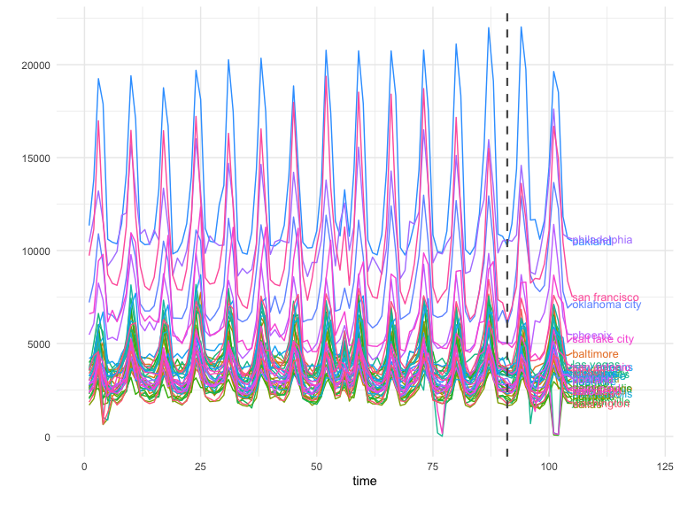
A good next step is to plot the panel data with GeoPlot to observe it’s trend, contribution per location, and also to detect any data anomalies before moving on to the data analysis.

GeoPlot(GeoTestData_PreTest,
        Y_id = "Y",
        time_id = "time",
        location_id = "location")

GeoPlot

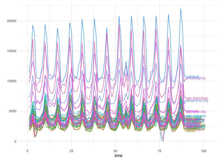
In this case we see a similar pattern that’s shared across all locations. These structural similarities between regions are the key to a successful test!

2. Power Analysis

Running a prospective power analysis is fundamental prior to executing a test. It is only through a thorough statistical analysis of our data that we can set it up for success. In general, through the power analysis we can find:

The optimal number of test locations.
Best test duration.
Select the ideal test and control markets.
Get a good estimate of the budget needed to run the test.
Determine which is the Minimum Detectable Effect to obtain significant results.
Align expectations.

Assessing the power and selecting the test markets for a GeoLift test can be accomplished through the GeoLiftMarketSelection() function. Through a series of simulations, this algorithm will find which are the best combinations of test and control locations for the experiment. Moreover, for each of these test market selections, the function will display the Minimum Detectable Effect, minimum investment needed to run a successful test, and other important model-fit metrics that will help us select the test that best matches our goals and resources.

The key parameters needed to run this function are:

data: A data frame containing the historical conversions by geographic unit. This object must contain at least a “location” column with the geo name, a “Y” column with the outcome data (such as units), a “time” column with the indicator of the time period (starting at 1), and covariates (if available). Using the data frame generated by GeoDataRead() is the best way to make sure we have the correct format. For this example, we will use GeoTestData_PreTest.
treatment_periods: List of treatment periods to calculate power for. If we’re unsure of the ideal test duration, we can specify and assess the power of different durations. The ideal test length heavily depends on the product and vertical we are working with. Nevertheless, a good rule of thumb when deciding duration is to make sure that the test period can contain at least one full purchase cycle. Given that we have daily data in our example, we will analyze the power of 10 and 15-day tests by setting this parameter to c(10,15).
N: List of number of test markets to calculate power for. The values in this list represent the different test-market sizes we want to explore. This parameter is often guided by the budget and scope of the test we want to implement. For our example, we will analyze smaller tests with two, three, and four test markets (the remaining would be part of the control). We will do so by setting this parameter to c(2,3,4).
X (Optional): List of the names of the covariates in the data. In our example we don’t have any covariates so we’ll leave it empty.
Y_id, location_id, and time_id: Names of the outcome, location, and time variables (String). These parameters will let our function know are the names of these variables in our data frame. If left empty, this parameter will default to the defaults of GeoDataRead() which are: Y, location, and time.
effect_size: This parameter contains a vector of different effect sizes (or lifts) we want to simulate. Since these are relative values, they do depend on the product and vertical we’re analyzing. For instance, while a small single-digit percent increase in volume for a retailer can translate to millions of units, a large lift might be required for an automotive company that sells fewer products per day. By default this parameter is set to a sequence of lifts between 0 and 25 percent with 5% increments, that is, seq(0,0.25,0.05).
lookback_window: A number indicating how far back in time the simulations for the power analysis should go. For instance, a value equal to 5 would simulate power for the last five possible tests. In general, when the historical data is stable (it doesn’t vary wildly from one day/region to another) we can obtain a very robust and reliable power analysis by just looking into the most recent possible test (in other words, lookback_window = 1). It is important to mention that increasing the values in this parameter can significantly increase the algorithm’s run-time.
include_markets: A list of markets or locations that should be part of the test group. Assuming that we need to have Chicago as part of our test regions, we will set this parameter to include_markets = c("chicago"). Make sure the spelling of locations in this lists matches with the data.
exclude_markets: A list of markets or locations that won’t be considered for the test market selection, but will remain in the pool of controls. In our example, we will set exclude_markets = c("honolulu") to make sure that only cities in the continental US will be part of the test group. As with include_locations, always make sure the spelling of locations in this lists matches with the data.
holdout: A vector with two values: the first one the smallest desirable holdout and the second the largest desirable holdout. The holdout represents the share of conversions from markets that will not see our ad campaign. In our example, will specify that we’re OK with a large holdout and will therefore set holdout = c(0.5, 1). If this parameter is left empty, all market selections will be analyzed regardless of their size.
cpic: Value indicating the Cost Per Incremental Conversion, that is, on average how much do we typically need to spend to bring one incremental conversion. CPIC estimates can typically be obtained from Marketing Mix Models, Conversion Lifts, and previous experiments/geo-experiments. This value is key to get a good estimate of the budget that we will need to run a well-powered test. If there is no reliable information about the Cost Per Incremental Conversion, the default will be set to cpic = 1, in which case, the investment results will output the incremental units needed for a successful test.
budget: Optional parameter that indicates the maximum budget available for a GeoLift test. If no budget is provided, all market selections will be analyzed by the algorithm.
alpha: This parameter controls the significance Level that will be used by our model. By default alpha = 0.1 which is equivalent to a 90% confidence level.
model: A string that indicates the outcome model used to augment the Augmented Synthetic Control Method. Augmentation through a prognostic function can improve fit and reduce L2 imbalance metrics. The most common values used are: model = "None" (default) which won’t augment the ASCM and model = "Ridge". More information on this parameter is given in the Inference section of this walkthrough.
fixed_effects: A logic flag indicating whether to include unit Fixed Effects (FE) in the model. Fixed effects are an additional parameter that we can include into our models which represents a non-random component in our data. More specifically, in our model the FE represents the “level” of each region’s time-series across the data. By adding the FE we effectively remove this level - this allows our model to focus on explaining the variations from that level rather than the full value of Y. This is helpful when the series are stable across time. However, if the series isn’t stable (it has large spikes/valleys, has a clear trend, etc.), then it can actually be a detriment to our model. By default, this parameter is set to fixed_effects = TRUE. A close inspection of GeoPlot’s output combined with knowledge of the data is key to specify this parameter. In our example, we will set fixed_effects = TRUE given that we can observe a stable behavior of sales across our markets in the historical data.
Correlations: A logic flag indicating whether an additional column to the output with the correlations between the test regions and control markets. Given that not all locations in the pool of controls will contribute meaningfully to create our counterfactual/synthetic test region, the correlations can be a great resource to know how representative our test region is which can inform other analyses such as Marketing Mix Model calibration. By default this parameter is set to Correlations = FALSE.
print: print A logic flag indicating whether to print the top results. Set to TRUE by default.
parallel: A logic flag indicating whether to use parallel computing to speed up calculations. Set to TRUE by default.
parallel_setup: A string indicating parallel workers set-up. Set to parallel_setup = "sequential" by default but can also be defined as parallel_setup = "parallel".
side_of_test: A string indicating whether confidence will be determined using a one sided or a two sided test. These are the following valid values for this parameter:
- side_of_test = "two_sided": The test statistic is the sum of all treatment effects, i.e. sum(abs(x)). Defualt.
- side_of_test = "one_sided": One-sided test against positive or negative effects i.e. If the effect being applied is negative, then defaults to -sum(x). If the effect being applied is positive, then defaults to sum(x).

Continuing with the example and in order to explore the function’s capabilities let’s assume we have two restrictions: Chicago must be part of the test markets and we have up to $100,000 to run the test. We can include these constraints into GeoLiftMarketSelection() with the include_markets and budget parameters and proceed with the market selection. Moreover, after observing that the historical KPI values in GeoPlot() have been stable across time we will proceed with a model with Fixed Effects. Finally, given a CPIC = $7.50 obtained from a previous Lift test, a range between two to five test markets, and a duration between 10 and 15 days we obtain:

    MarketSelections <- GeoLiftMarketSelection(data = GeoTestData_PreTest,
                                              treatment_periods = c(10,15),
                                              N = c(2,3,4,5),
                                              Y_id = "Y",
                                              location_id = "location",
                                              time_id = "time",
                                              effect_size = seq(0, 0.5, 0.05),
                                              lookback_window = 1,
                                              include_markets = c("chicago"),
                                              exclude_markets = c("honolulu"),
                                              holdout = c(0.5, 1),
                                              cpic = 7.50,
                                              budget = 100000,
                                              alpha = 0.1,
                                              Correlations = TRUE,
                                              fixed_effects = TRUE,
                                              side_of_test = "two_sided")

    ## Setting up cluster.
    ## Importing functions into cluster.
    ##
    ## Deterministic setup with 2 locations in treatment.
    ##
    ## Deterministic setup with 3 locations in treatment.
    ##
    ## Deterministic setup with 4 locations in treatment.
    ##
    ## Deterministic setup with 5 locations in treatment.
    ##   ID                                           location duration EffectSize
    ## 1  1             chicago, cincinnati, houston, portland       15       0.05
    ## 2  2                                  chicago, portland       15       0.10
    ## 3  3             chicago, cincinnati, houston, portland       10       0.10
    ## 4  4                                  chicago, portland       10       0.10
    ## 5  5                         chicago, houston, portland       10       0.10
    ## 6  6 chicago, cincinnati, houston, nashville, san diego       15       0.05
    ##   Power AvgScaledL2Imbalance Investment   AvgATT Average_MDE ProportionTotal_Y
    ## 1     1            0.1971864   74118.38 159.3627  0.04829913        0.07576405
    ## 2     1            0.1738778   64563.75 290.0071  0.10117316        0.03306537
    ## 3     1            0.1966996   99027.75 316.6204  0.09552879        0.07576405
    ## 4     1            0.1682310   43646.25 300.9401  0.10378013        0.03306537
    ## 5     1            0.2305628   75389.25 350.3142  0.10502968        0.05797087
    ## 6     1            0.2699167   95755.50 146.7975  0.04282215        0.09801138
    ##   abs_lift_in_zero   Holdout rank correlation
    ## 1            0.002 0.9242359    1   0.9144814
    ## 2            0.001 0.9669346    1   0.9321104
    ## 3            0.004 0.9242359    3   0.9144814
    ## 4            0.004 0.9669346    3   0.9321104
    ## 5            0.005 0.9420291    5   0.9139549
    ## 6            0.007 0.9019886    6   0.8992280

The results of the power analysis and market selection provide us with several key metrics that we can use to select our test market. These metrics are:

ID: Numeric ID that identifies a combination of test markets for a given duration. This variable will be useful to plot the results.
location: Identifies the test locations.
duration: Shows how many time-stamps the test will last for. Since the data in our example had daily values, we will analyze whether a 10 or 15 day test is ideal.
EffectSize: The Effect Size represents minimum Lift needed to have a well-powered test. These values depend on the effect_size parameter of this function. Therefore, if you see multiple ties across top candidates for our test markets, then it might be a good idea to increase the granularity in this parameter (for example to seq(0, 0.25, 0.01)).
Power: The row’s average power across all simulations at the specified Effect Size.
AvgScaledL2Imbalance: The Scaled L2 Imbalance metric is a goodness of fit metric between 0 and 1 that represents how well the model is predicting the pre-treatment observed values through the Synthetic Control. Scaled L2 Imbalance values of 0 show a perfect match of pre-treatment values. Scaled L2 Imbalance values of 1 show that the Synthetic Control algorithm is not adding much value beyond what you could accomplish with a simple average of control locations (naive model).
Investment: The average investment needed to obtain a well-powered test given a CPIC.
AvgATT: The ATT is a metric of how many incremental units, on average, our test markets will have across each time-stamp for the duration of the test for a given set of test markets, duration, and Effect Size.
Average_MDE: The average Minimum Detectable Effect across all simulations.
ProportionTotal_Y: This proportion reflects the fraction of all conversions that happen in our test regions compared to the aggregation of all markets. For example, a value of 0.10 would indicate that our test markets represent 10% of all conversions for our KPI.
abs_lift_in_zero: This value represents the average estimated lift our test markets had when we actually simulated a 0% Lift in conversions. Great test market selections often have values of abs_lift_in_zero very close to zero.
Holdout: The percent of total conversions in the control markets. This value is complementary to ProportionTotal_Y.
rank: Ranking variable that summarizes the EffectSize, Power, AvgScaledL2Imbalance, Average_MDE, and abs_lift_in_zero to help you select the best combination of test markets. The ranking variable allows for ties.

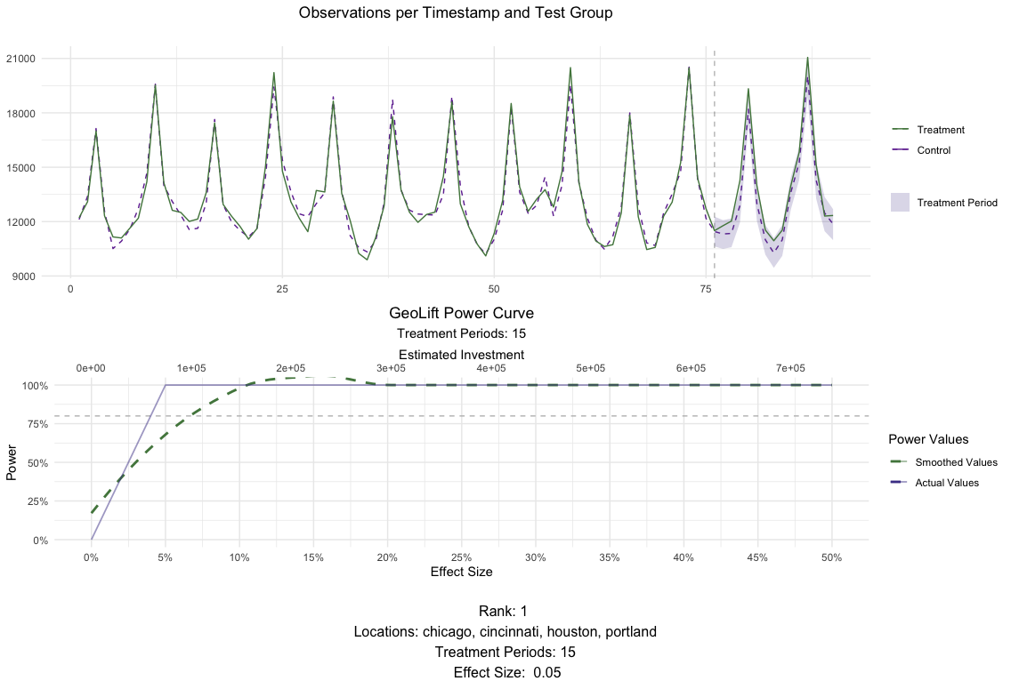
The results in MarketSelection show that the test markets with the best ranks are: (chicago, cincinnati, houston, portland) and (chicago, portland), both tied at rank 2. We can plot() both of these results to inspect them further. This plot will show how the results of the GeoLift() model would look like with the latest possible test period as well as the test’s power curve across all simulations.

    # Plot for chicago, cincinnati, houston, portland for a 15 day test
    plot(MarketSelections, market_ID = 1, print_summary = FALSE)

GeoPlot

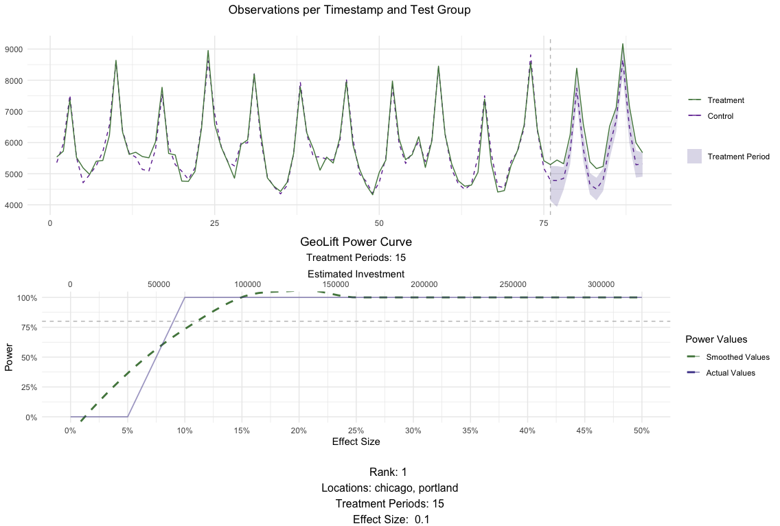
    # Plot for chicago, portland for a 15 day test
    plot(MarketSelections, market_ID = 2, print_summary = FALSE)

GeoPlot

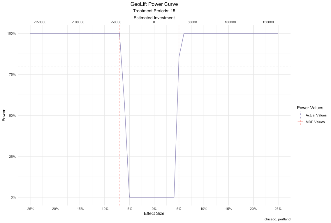
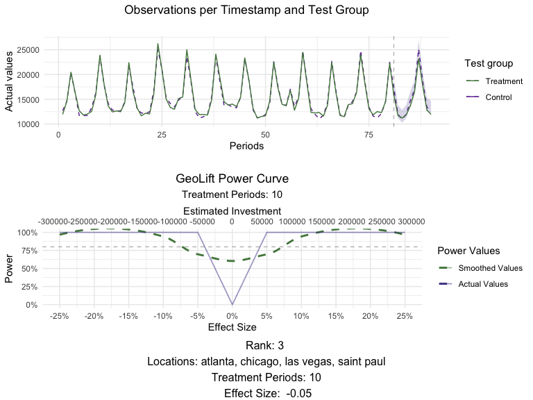
Power output - deep dive into power curves

In order to ensure that power is consistent throughout time for these locations, we can run more than 1 simulation for each of the top contenders that came out of GeoLiftMarketSelection.

We will do this by running the GeoLiftPower method and expanding our lookback_window to 7 days, only for this treatment combination and plot their results.

NOTE: You could repeat this process for the top 5 treatment combinations that come out of GeoLiftMarketSelection, with increased lookback windows and compare their power curves. We will do it only for Chicago and Portland here.

market_id = 2
market_row <- MarketSelections$BestMarkets %>% dplyr::filter(ID == market_id)
treatment_locations <- stringr::str_split(market_row$location, ", ")[[1]]
treatment_duration <- market_row$duration
lookback_window <- 7

power_data <- GeoLiftPower(
  data = GeoTestData_PreTest,
  locations = treatment_locations,
  effect_size = seq(-0.25, 0.25, 0.01),
  lookback_window = lookback_window,
  treatment_periods = treatment_duration,
  cpic = 7.5,
  side_of_test = "two_sided"
)
#> Setting up cluster.
#> Importing functions into cluster.

plot(power_data, show_mde = TRUE, smoothed_values = FALSE, breaks_x_axis = 5) +
    labs(caption = unique(power_data$location))

GeoLiftPowerTopContenders

While both market selections perform excellent on all metrics, we will move further with the latter since it allows us to run a successful test with a smaller budget. Finally, changing the print_summary parameter of plot() to TRUE can provide us with additional information about this market selection.

    # Plot for chicago, portland for a 15 day test
    plot(MarketSelections, market_ID = 2, print_summary = TRUE)

    ## ##################################
    ## #####   GeoLift Simulation   #####
    ## ####  Simulating: 10% Lift  ####
    ## ##################################
    ##
    ## GeoLift Results Summary
    ## ##################################
    ## #####     Test Statistics    #####
    ## ##################################
    ##
    ## * Average ATT: 290.007
    ## * Percent Lift: 10.1%
    ## * Incremental Y: 8700
    ## * P-value: 0
    ##
    ## ##################################
    ## #####   Balance Statistics   #####
    ## ##################################
    ##
    ## * L2 Imbalance: 868.598
    ## * Scaled L2 Imbalance: 0.1739
    ## * Percent improvement from naive model: 82.61%
    ## * Average Estimated Bias: NA
    ##
    ## ##################################
    ## #####     Model Weights      #####
    ## ##################################
    ##
    ## * Prognostic Function: NONE
    ##
    ## * Model Weights:
    ##  * cincinnati: 0.2429
    ##  * miami: 0.2056
    ##  * baton rouge: 0.1511
    ##  * honolulu: 0.0669
    ##  * dallas: 0.0644
    ##  * nashville: 0.0641
    ##  * minneapolis: 0.0619
    ##  * san diego: 0.0394
    ##  * houston: 0.0292
    ##  * austin: 0.0237
    ##  * new york: 0.0216
    ##  * los angeles: 0.0179
    ##  * reno: 0.0113

GeoPlot

Note: Given that we are not using the complete pre-treatment data to calculate the weights in our power analysis simulations, the ones displayed by the plotting function above are not the final values. However, you can easily obtain them with the `GetWeights()` function.

    weights <- GetWeights(Y_id = "Y",
                          location_id = "location",
                          time_id = "time",
                          data = GeoTestData_PreTest,
                          locations = c("chicago", "portland"),
                          pretreatment_end_time = 90,
                          fixed_effects = TRUE)
    #> One outcome and one treatment time found. Running single_augsynth.

    # Top weights
    head(dplyr::arrange(weights, desc(weight)))
    #>      location     weight
    #> 1  cincinnati 0.22717797
    #> 2       miami 0.20276981
    #> 3 baton rouge 0.13353743
    #> 4 minneapolis 0.08997973
    #> 5      dallas 0.07392298
    #> 6   nashville 0.06853184

3. Analyzing the Test Results

Based on the results of the Power Calculations, a test is set-up in which a 15-day marketing campaign will be executed in the cities of Chicago and Portland while the rest of the locations will be put on holdout. Following the completion from this marketing campaign, we receive sales data that reflects these results. This new data-set contains the same format and information as the pre-test one but crucially includes results for the duration of the campaign. Depending on the vertical and product, adding a post-campaign cooldown period might be useful.

Test Data

Data for the campaign results can be accessed at GeoLift_Test.

data(GeoLift_Test)

Similarly to the process executed at the beginning of the Power Analysis phase, we read the data into GeoLift’s format using the GeoDataRead function. You can observe in the summary output that additional 15 periods are contained in the new GeoLift data object.

    GeoTestData_Test <- GeoDataRead(data = GeoLift_Test,
                                        date_id = "date",
                                        location_id = "location",
                                        Y_id = "Y",
                                        X = c(), #empty list as we have no covariates
                                        format = "yyyy-mm-dd",
                                        summary = TRUE)

    #> ##################################
    #> #####       Summary       #####
    #> ##################################
    #>
    #> * Raw Number of Locations: 40
    #> * Time Periods: 105
    #> * Final Number of Locations (Complete): 40
``` r
    head(GeoTestData_Test)
    #>   location time    Y
    #> 1  atlanta    1 3384
    #> 2  atlanta    2 3904
    #> 3  atlanta    3 5734
    #> 4  atlanta    4 4311
    #> 5  atlanta    5 3686
    #> 6  atlanta    6 3374

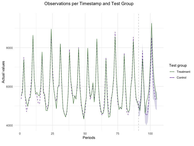
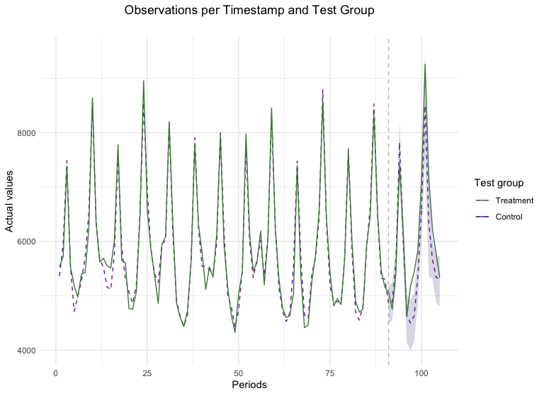
The results can also be plotted using the GeoPlot function. However, for post-campaign data we can include the time-stamp at which the campaign started through the treatment_start parameter to clearly separate the two periods. Plotting the time-series is always useful to detect any anomalies with the data and to start noticing patterns with the test.

GeoPlot(GeoTestData_Test,
        Y_id = "Y",
        time_id = "time",
        location_id = "location",
        treatment_start = 91)

GeoPlotTestData

GeoLift Inference

The next step in the process is to calculate the actual Lift caused by the marketing campaigns on our test locations. To do so we make use of the GeoLift() function, which will take as input the GeoLift dataframe as well as information about the test such as which were the cities in the treatment group, when the test started, and when it ended through the locations, treatment_start_time, and treatment_end_time parameters respectively.

    GeoTest <- GeoLift(Y_id = "Y",
                        data = GeoTestData_Test,
                        locations = c("chicago", "portland"),
                        treatment_start_time = 91,
                        treatment_end_time = 105)

    GeoTest

    #> One outcome and one treatment time found. Running single_augsynth.
    #>
    #> GeoLift Output
    #>
    #> Test results for 15 treatment periods, from time-stamp 91 to 105 for test markets:
    #> 1 CHICAGO
    #> 2 PORTLAND
    #> ##################################
    #> #####     Test Statistics    #####
    #> ##################################
    #>
    #> Percent Lift: 5.4%
    #>
    #> Incremental Y: 4667
    #>
    #> Average Estimated Treatment Effect (ATT): 155.556
    #>
    #> The results are significant at a 95% level. (TOTAL)
    #>
    #> There is a 0.6% chance of observing an effect this large or larger assuming treatment effect is zero.

The results show that the campaigns led to a 5.4% lift in units sold corresponding to 4667 incremental units for this 15-day test. Moreover, the Average Estimated Treatment Effect is of 155.556 units every day of the test. Most importantly, we observe that these results are statistically significant at a 95% level. In fact, there’s only a 0.6% chance of observing an effect of this magnitude or larger if the actual treatment effect was zero. In other words, it is extremely unlikely that these results are just due to chance. To dig deeper into the results, we can run the summary() of our GeoLift object.

    summary(GeoTest)

    #>
    #> GeoLift Results Summary
    #> ##################################
    #> #####     Test Statistics    #####
    #> ##################################
    #>
    #> * Average ATT: 155.556
    #> * Percent Lift: 5.4%
    #> * Incremental Y: 4667
    #> * P-value: 0.01
    #>
    #> ##################################
    #> #####   Balance Statistics   #####
    #> ##################################
    #>
    #> * L2 Imbalance: 909.489
    #> * Scaled L2 Imbalance: 0.1636
    #> * Percent improvement from naive model: 83.64%
    #> * Average Estimated Bias: NA
    #>
    #> ##################################
    #> #####     Model Weights      #####
    #> ##################################
    #>
    #> * Prognostic Function: NONE
    #>
    #> * Model Weights:
    #>  * austin: 0.0465
    #>  * baton rouge: 0.1335
    #>  * cincinnati: 0.2272
    #>  * dallas: 0.0739
    #>  * honolulu: 0.0673
    #>  * houston: 0.0046
    #>  * miami: 0.2028
    #>  * minneapolis: 0.09
    #>  * nashville: 0.0685
    #>  * new york: 0.0046
    #>  * reno: 0.0306
    #>  * san antonio: 0.0054
    #>  * san diego: 0.0451

The summary show additional test statistics such as the p-value which was equal to 0.01 confirming the highly statistical significance of these results. Moreover, the summary function provides Balance Statistics which display data about our model’s fit. The main metric of model fit used in GeoLift is the L2 Imbalance which represents how far our synthetic control was from the actual observed values in the pre-treatment period. That is, how similar the synthetic Chicago + Portland unit we crated is from the observed values of these cities in the period before the intervention. A small L2 Imbalance score means that our model did a great job replicating our test locations while a large one would indicate a poor fit. However, the L2 Imabalnce metric is scale-dependent, meaning that it can’t be compared between models with different KPIs or number of testing periods. For instance, the L2 Imbalance of a model run on grams of units sold will be significantly larger than a model ran for tons of product sold even if they represent the same basic underlying metric.

Therefore, given that it’s hard to tell whether the model had a good or poor fit by simply looking at the value of the L2 Imbalance metric, we also included the Scaled L2 Imbalance stat which is easier to interpret as it’s bounded in the range between 0 and 1. A value close to zero represents a good model fit while values nearing 1 indicate a poor performance by the Synthetic Control Model. This scaling is accomplished by comparing the Scaled L2 Imbalance of our Synthetic Control Method with the Scaled L2 Imbalance obtained by a baseline/naive model (instead of carefully calculating which is the optimal weighting scheme for the Synthetic Control, we assign equal weights to each unit in the donor pool). The latter provides an upper bound of L2 Imbalance, therefore, the Scaled L2 Imbalance shows us how much better our GeoLift model is from the baseline.

In fact, another way to look at the Scaled L2 Imbalance is the percent improvement from a naive model which can be obtained by subtracting our model’s Scaled L2 Imbalance from 100%. In this case, an improvement close to 100% (which corresponds to a Scaled L2 Imbalance close to zero) represents a good model fit. Finally, we also include the weights that generate our Synthetic Control. In this test we note that the locations that contribute the most to our GeoLift model are Cincinnati, Miami, and Baton Rouge.

    plot(GeoTest, type = "Lift")
    #> You can include dates in your chart if you supply the end date of the treatment. Just specify the treatment_end_date parameter.

LiftPlot

Plotting the results is a great way to assess the model’s fit and how effective the campaign was. Taking a close look at the pre-treatment period (period before the dotted vertical line) provides insight into how well our Synthetic Control Model fitted our data. In this specific example, we see that the observed values of the Chicago + Portland test represented in the solid black line were closely replicated by our SCM model shown as the dashed red line. Furthermore, looking at the test period, we can notice the campaign’s incrementality shown as the difference between the sales observed in the test markets and our counterfactual synthetic location. This marked difference between an almost-exact match in pre-treatment periods and gap in test time-stamps provides strong evidence of a successful campaign.

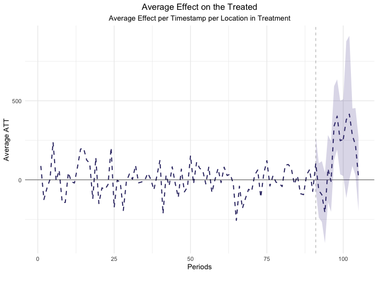
    plot(GeoTest, type = "ATT")
    #> You can include dates in your chart if you supply the end date of the treatment. Just specify the treatment_end_date parameter.

PlotATT

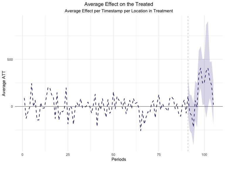
Looking at the Average Estimated Treatment Effect’s plot can also be extremely useful. The ATT metric shows us the magnitude of the Average Treatment Effect on a daily basis in contrast with the previous (Lift) plot which focused on aggregated effects. Moreover, this is a great example of a good GeoLift model as it has very small ATT values in the pre-treatment period and large ones when the treatment is administered to our test locations. Moreover, point-wise confidence intervals are included in this chart which help us measure how significant each day’s Lift has been.

Improving The Model

While the results obtained from the test are robust and highly significant, a useful feature of GeoLift is its ability to improve the model fit even further and reduce bias through augmentation by a prognostic function. There are several options for augmentation of the standard GeoLift model such as regularization (specifically Ridge) and an application of Generalized Synthetic Control Model (GSC). While each of these approaches provide it’s own set of advantages, for instance Ridge regularization usually performs well when the number of units and time-periods isn’t large while GSC helps improve fit for situations with many pre-treatment periods, GeoLift offers the option to let the model decide which is the best approach by setting the model parameter to “best”.

    GeoTestBest <- GeoLift(Y_id = "Y",
                            data = GeoTestData_Test,
                            locations = c("chicago", "portland"),
                            treatment_start_time = 91,
                            treatment_end_time = 105,
                            model = "best")

    #> One outcome and one treatment time found. Running single_augsynth.
    #> One outcome and one treatment time found. Running single_augsynth.
    #> One outcome and one treatment time found. Running single_augsynth.
    #> One outcome and one treatment time found. Running single_augsynth.
    #>
    #> GeoLift Output
    #>
    #> Test results for 15 treatment periods, from time-stamp 91 to 105 for test markets:
    #> 1 CHICAGO
    #> 2 PORTLAND
    #> ##################################
    #> #####     Test Statistics    #####
    #> ##################################
    #>
    #> Percent Lift: 5.5%
    #>
    #> Incremental Y: 4704
    #>
    #> Average Estimated Treatment Effect (ATT): 156.805
    #>
    #> The results are significant at a 95% level. (TOTAL)
    #>
    #> There is a 1.4% chance of observing an effect this large or larger assuming treatment effect is zero.

    summary(GeoTestBest)

    #>
    #> GeoLift Results Summary
    #> ##################################
    #> #####     Test Statistics    #####
    #> ##################################
    #>
    #> * Average ATT: 156.805
    #> * Percent Lift: 5.5%
    #> * Incremental Y: 4704
    #> * P-value: 0.01
    #>
    #> ##################################
    #> #####   Balance Statistics   #####
    #> ##################################
    #>
    #> * L2 Imbalance: 903.525
    #> * Scaled L2 Imbalance: 0.1626
    #> * Percent improvement from naive model: 83.74%
    #> * Average Estimated Bias: -1.249
    #>
    #> ##################################
    #> #####     Model Weights      #####
    #> ##################################
    #>
    #> * Prognostic Function: RIDGE
    #>
    #> * Model Weights:
    #>  * atlanta: 3e-04
    #>  * austin: 0.0467
    #>  * baltimore: 1e-04
    #>  * baton rouge: 0.1337
    #>  * boston: -4e-04
    #>  * cincinnati: 0.2273
    #>  * columbus: 1e-04
    #>  * dallas: 0.0741
    #>  * denver: 1e-04
    #>  * detroit: 1e-04
    #>  * honolulu: 0.0674
    #>  * houston: 0.0048
    #>  * indianapolis: 1e-04
    #>  * jacksonville: -1e-04
    #>  * kansas city: -1e-04
    #>  * los angeles: 2e-04
    #>  * memphis: -2e-04
    #>  * miami: 0.2029
    #>  * milwaukee: -2e-04
    #>  * minneapolis: 0.0901
    #>  * nashville: 0.0687
    #>  * new orleans: -2e-04
    #>  * new york: 0.0048
    #>  * oakland: -0.001
    #>  * oklahoma city: -7e-04
    #>  * orlando: 1e-04
    #>  * philadelphia: -4e-04
    #>  * reno: 0.0308
    #>  * saint paul: 2e-04
    #>  * salt lake city: -3e-04
    #>  * san antonio: 0.0056
    #>  * san diego: 0.0452
    #>  * san francisco: 1e-04
    #>  * tucson: -1e-04

    plot(GeoTestBest, type = "Lift")
    #> You can include dates in your chart if you supply the end date of the treatment. Just specify the treatment_end_date parameter.

PlotLiftBest

    plot(GeoTestBest, type = "ATT")
    #> You can include dates in your chart if you supply the end date of the treatment. Just specify the treatment_end_date parameter.

PlotATTBest

The new results augment the GeoLift model with a Ridge prognostic function which improves the model fit as seen in the new L2 Imbalance metrics. This additional robustness is translated in a small increase in the Percent Lift. Furthermore, by augmenting the model with a prognostic function, we have an estimate of the estimated bias that was removed by the Augmented Synthetic Control Model.

1. Data and R Environment​

Set-up of the R Environment​

Data​

Note: Before reading the data into this format, always make sure that there are no missing variables, NAs, or locations with missing time-stamps as those will be dropped by the GeoDataRead() function.​

2. Power Analysis​

Power output - deep dive into power curves​

NOTE: You could repeat this process for the top 5 treatment combinations that come out of GeoLiftMarketSelection, with increased lookback windows and compare their power curves. We will do it only for Chicago and Portland here.​

Note: Given that we are not using the complete pre-treatment data to calculate the weights in our power analysis simulations, the ones displayed by the plotting function above are not the final values. However, you can easily obtain them with the GetWeights() function.​

3. Analyzing the Test Results​

Test Data​

GeoLift Inference​

Improving The Model​

1. Data and R Environment

Set-up of the R Environment

Data

Note: Before reading the data into this format, always make sure that there are no missing variables, `NAs`, or locations with missing time-stamps as those will be dropped by the `GeoDataRead()` function.

2. Power Analysis

Power output - deep dive into power curves

NOTE: You could repeat this process for the top 5 treatment combinations that come out of GeoLiftMarketSelection, with increased lookback windows and compare their power curves. We will do it only for Chicago and Portland here.

Note: Given that we are not using the complete pre-treatment data to calculate the weights in our power analysis simulations, the ones displayed by the plotting function above are not the final values. However, you can easily obtain them with the `GetWeights()` function.

3. Analyzing the Test Results

Test Data

GeoLift Inference

Improving The Model