Multi-Cell Walkthrough
Introduction to Multi-Cell GeoLifts
One of the key competitive advantages of Geo-Experimental techniques such as GeoLift is that they can empower decision-makers to make apples-to-apples comparisons across different channels. Multi-Cell experiments on GeoLift take this concept to the next level by allowing users to easily set-up and analyze complex experimental designs where more than one channel or strategy is measured simultaneously. With Multi-Cell GeoLifts you can:
- Compare the incremental effect and ROI of two or more channels.
- Improve a channel's strategy by evaluating which of two or more implementations provides better business results.
- Optimize your media mix based on data and science!
Multi-Cell Tests with GeoLift
Starting on v2.5 of GeoLift, a new set of functions were introduced to run Multi-Cell tests. In this context, each cell refers to a different test group which will be used to measure and compare across strategies or channels. After identifying the KPI that will be measured with the experiment, the typical flow of a Multi-Cell experiment is as follows:
Determine how many cells or test groups will be used in the experiment.
Run
MultiCellMarketSelectionwith the pre-determined number of cells (k). This function will returnkoptimal simultaneous test groups.Use
MultiCellPowerto obtain a detailed Power Curve and required investment for each cell.
- [Optional]:
MultiCellWinnercan provide valuable information if the test's objective is to determine whether a strategy/channel is statistically significantly better than the others. The output of this function will specify what would be needed for a cell to be declared winner based on statistical tests of equivalence.
Run the campaigns.
Run inference with
GeoLiftMultiCell, find out the true incremental value of each cell, conclude whether there was a winner, and use the results to optimize your strategy!
After downloading GeoLift v2.5 (or greater), the first step is to load the package:
# Load libraries
library(GeoLift)
library(dplyr)
1. Determining the number of Cells
Figuring out how many cells will be measured in a GeoLift test is a crucial first step in the Multi-Cell process. Here, it is important to take into consideration that each cell will be measured by one or more test regions (city, state, DMA, etc.). Therefore, the total number of cells that can be measured with a GeoLift is bounded by the available data. Our recommendation is to be very conservative with the number of cells in a single GeoLift study.
For this Walkthrough we will explore a cross-channel test to measure and compare the Lift of our largest Social Media and Paid Search channels. We will use the sample data included in this package:
data(GeoLift_PreTest)

# Read into GeoLifts format with GeoDataRead
GeoTestData_PreTest <- GeoDataRead(data = GeoLift_PreTest,
                                    date_id = "date",
                                    location_id = "location",
                                    Y_id = "Y",
                                    X = c(), #empty list as we have no covariates
                                    format = "yyyy-mm-dd",
                                    summary = TRUE)

# Plot the KPI's historical values
GeoPlot(GeoTestData_PreTest)
The dataset contains the pre-treatment daily sales for 40 US cities across 90 days. The data-frame contains three variables: location (city), date (in “yyyy-mm-dd” format), and Y (number of conversions/KPI in each day/location).
Finally, it is important to highlight the trade-off between number of cells in a Multi-Cell GeoLift test and the model fit. Given that increasing the number of cells necessarily decreases the total available units in the pool of controls, adding too many cells can significantly reduce the model fit and accuracy. In our example, given that we only have 40 cities in total, it would be advisable to not run a Multi-Cell test with more than 2 or 3 cells.
2. Finding test markets with MultiCellMarketSelection
Once the number of cells, k, is determined, we can proceed to find the optimal test markets for each cell through MultiCellMarketSelection(). Relying on a sampling method defined by the user, the algorithm will create k similar groups. For each group, the algorithm will run a series of simulations to determine the best combinations of test and control locations.
The key parameters needed to run this function are:
data: A data frame containing the historical conversions by geographic unit. This object must contain at least: a “location” column with the geo name, a “Y” column with the outcome data (such as units), a “time” column with the indicator of the time period (starting at 1), and covariates (if available). Using the data frame generated byGeoDataRead()is the best way to make sure we have the correct format. For this example, we will useGeoTestData_PreTest.k: The number of partitions or cells. For our example we will analyze ak = 2corresponding to the Social Media and Search channels.sampling_method: Sampling method used to create thekpartitions in the data set. At the moment, only systematic sampling (sampling_method = 'systematic') is available, but more options will be added in the future.top_choices: Specifies the number of top markets per cell to be displayed by the output.N: List of number of test markets to calculate power for. The values in this list represent the different test-market sizes we want to explore for each cell. This parameter is often guided by the budget and scope of the test we want to implement. For our example, we will analyze smaller tests with two and three test markets per cell (the remaining would be part of the control). We will do so by setting this parameter toc(2,3).X(Optional): List of the names of the covariates in the data. In our example we don’t have any covariates so we’ll leave it empty.Y_id,location_id, andtime_id: Names of the outcome, location, and time variables. These parameters will let our function know are the names of these variables in our data frame. If left empty, this parameter will default to the standard values provided byGeoDataRead()which are:Y,location, andtime.effect_size: This parameter contains a vector of different effect sizes (or lifts) we want to simulate. For simplicity of analysis, we strongly recommend focusing on either all positive or negative values for this parameter. For this example, we will set this parameter to a sequence of lifts between 0 and 25 percent with 2.5% increments, that is, seq(0,0.25,0.025).treatment_periods: Specifies the test length. We recommend to specify a single treatment length for Multi-cell GeoLift Market Selections. In this example, we will analyze a 15-day test so we will settreatment_periods = c(15).lookback_window: A number indicating how far back in time the simulations for the power analysis should go. For instance, a value equal to 7 would simulate power for the last seven days. In general, when the historical data is stable (it doesn’t vary wildly from one day/region to another) we can obtain a very robust and reliable power analysis by just looking into the most recent possible test (in other words,lookback_window = 1). It is important to mention that increasing the values in this parameter can significantly increase the algorithm’s run-time. A common best practice is to keeplookback_window = 1forMultiCellMarketSelectionand then increasing it if needed in the next step of the Multi-Cell process.cpic: List of values indicating the Cost Per Incremental Conversion per cell, that is, on average how much do we typically need to spend to bring one incremental conversion. CPIC estimates can typically be obtained from Marketing Mix Models, Conversion Lifts, and previous experiments/geo-experiments. This value is key to get a good estimate of the budget that we will need to run a well-powered test. If there is no reliable information about the Cost Per Incremental Conversion, the default will be set tocpic = 1, in which case, the investment results will output the incremental units needed for a successful test. If the KPI measured is in a currency rather than in units, then it should be set as the inverse of the incremental Return on Ad Spend (cpic = 1/iROAS). In this example, considering that our KPI is in units we will use acpic = c(7.50,7.00)for the Social Media and Paid Search cells respectively. Thesecpicvalues were guided by the results of previous single-cell GeoLifts.alpha: This parameter controls the significance Level that will be used by our model. By defaultalpha = 0.1which is equivalent to a 90% confidence level.model: A string that indicates the outcome model used to augment the Augmented Synthetic Control Method. Augmentation through a prognostic function can improve fit and reduce L2 imbalance metrics. The most common values used are:model = "None"(default) which won’t augment the ASCM andmodel = "Ridge".fixed_effects: A logic flag indicating whether to include unit Fixed Effects (FE) in the model. Fixed effects are an additional parameter that we can include into our models which represents a non-random component in our data. More specifically, in our model the FE represents the “level” of each region’s time-series across the data. By adding the FE we effectively remove this level - this allows our model to focus on explaining the variations from that level rather than the full value of Y. This is helpful when the series are stable across time. However, if the series isn’t stable (it has large spikes/valleys, has a clear trend, etc.), then it can actually be a detriment to our model. By default, this parameter is set to fixed_effects = TRUE. A close inspection of GeoPlot’s output combined with knowledge of the data is key to specify this parameter. In our example, we will set fixed_effects = TRUE given that we can observe a stable behavior of sales across our markets in the historical data.Correlations: A logic flag indicating whether an additional column to the output with the correlations between the test regions and control markets. Given that not all locations in the pool of controls will contribute meaningfully to create our counterfactual/synthetic test region, the correlations can be a great resource to know how representative our test region is which can inform other analyses such as Marketing Mix Model calibration.side_of_test: A string indicating whether confidence will be determined using a one sided or a two sided test. These are the following valid values for this parameter:side_of_test = "two_sided": The test statistic is the sum of all treatment effects.side_of_test = "one_sided": One-sided test against positive or negative effects.
Taking this inputs into consideration, we find:
set.seed(8) #To replicate the results
Markets <- MultiCellMarketSelection(data = GeoTestData_PreTest,
                                 k = 2,
                                 sampling_method = "systematic",
                                 top_choices = 10,
                                 N = c(2,3),
                                 effect_size = seq(0, 0.25, 0.025),
                                 treatment_periods = c(15),
                                 lookback_window = 1,
                                 cpic = c(7, 7.50),
                                 alpha = 0.1,
                                 model = "None",
                                 fixed_effects = TRUE,
                                 Correlations = TRUE,
                                 side_of_test = "one_sided")
Markets

##    cell ID                            location duration EffectSize
## 1     1  1                 chicago, cincinnati       15      0.025
## 2     2  1                     baltimore, reno       15      0.025
## 3     1  2            cleveland, oklahoma city       15      0.050
## 4     2  2                       houston, reno       15      0.025
## 5     1  3               las vegas, saint paul       15      0.025
## 6     2  3              honolulu, indianapolis       15      0.025
## 7     1  4                nashville, san diego       15      0.025
## 8     2  4             houston, portland, reno       15      0.025
## 9     1  5               philadelphia, phoenix       15      0.025
## 10    2  5         denver, memphis, washington       15      0.050
## 11    1  6    cleveland, dallas, oklahoma city       15      0.025
## 12    2  6               baton rouge, portland       15      0.025
## 13    1  7               detroit, jacksonville       15      0.025
## 14    2  7                     denver, memphis       15      0.050
## 15    1  8         atlanta, chicago, nashville       15      0.050
## 16    2  8                 memphis, washington       15      0.025
## 17    1  9                  atlanta, nashville       15      0.050
## 18    2  9      baton rouge, houston, portland       15      0.025
## 19    1 10 columbus, jacksonville, minneapolis       15      0.025
## 20    2 10                     miami, portland       15      0.075
##    AvgScaledL2Imbalance abs_lift_in_zero Investment ProportionTotal_Y   Holdout
## 1             0.2587293            0.001   15548.58        0.03418832 0.9658117
## 2             0.3202672            0.002   20166.19        0.04151842 0.9584816
## 3             0.5582169            0.001   60865.35        0.06599073 0.9340093
## 4             0.4149685            0.003   20507.62        0.04282716 0.9571728
## 5             0.7667228            0.003   20827.62        0.04571975 0.9542802
## 6             0.3044968            0.004   16648.88        0.03307948 0.9669205
## 7             0.4379696            0.005   17827.78        0.03891756 0.9610824
## 8             0.2643562            0.005   28790.25        0.05949740 0.9405026
## 9             0.5666373            0.007   45695.48        0.09829630 0.9017037
## 10            0.6200586            0.008   57326.25        0.05922727 0.9407727
## 11            0.6198624            0.008   36378.83        0.07923764 0.9207624
## 12            0.2284603            0.010   16299.00        0.03289916 0.9671008
## 13            0.3317333            0.008   13281.10        0.02940561 0.9705944
## 14            0.6591485            0.009   42621.00        0.04433701 0.9556630
## 15            0.5302774            0.008   55532.05        0.06089060 0.9391094
## 16            0.4803747            0.011   19126.69        0.03939854 0.9606015
## 17            0.6205455            0.008   40863.20        0.04449547 0.9555045
## 18            0.2413871            0.015   28416.38        0.05780466 0.9421953
## 19            0.3246004            0.010   24523.98        0.05485904 0.9451410
## 20            0.3733400            0.010   50877.56        0.03495877 0.9650412
##    rank
## 1     1
## 2     1
## 3     2
## 4     2
## 5     2
## 6     3
## 7     4
## 8     4
## 9     5
## 10    5
## 11    6
## 12    6
## 13    6
## 14    6
## 15    8
## 16    8
## 17    8
## 18    9
## 19    8
## 20    9
The resulting table contains optimal test designs for this two-cell test as well as some model-fit metrics for each selection. The columns in the results represent:
- cell: Numeric identifier for each cell. In our case, we have two cells: cell one for Social Media and cell 2 for Paid Search.
- ID: Numeric identifier of a test market for a given duration. The combination of cell and ID completely defines a Multi-Cell market selection.
- location: Identifies the test location(s).
- duration: Shows how many time-stamps the test will last for. Since the data in our example had daily values, we will analyze a 15 day test.
- EffectSize: The Effect Size represents minimum Lift needed to have a well-powered test. These values directly depend on the
effect_sizeparameter of this function. - Power: The row’s average power across all simulations at the specified Effect Size.
- AvgScaledL2Imbalance: The Scaled L2 Imbalance metric is a goodness of fit metric between 0 and 1 that represents how well the model is predicting the pre-treatment observed values through the Synthetic Control. Scaled L2 Imbalance values of 0 show a perfect match of pre-treatment values. Scaled L2 Imbalance values of 1 show that the Synthetic Control algorithm is not adding much value beyond what you could accomplish with a simple average of control locations (naive model).
- abs_lift_in_zero: This value represents the average estimated Lift our test markets had when we actually simulated a 0% Lift in conversions. Great test market selections often have values of abs_lift_in_zero very close to zero.
- Investment: The average investment needed to obtain a well-powered test given each cell's CPIC.
- ProportionTotal_Y: This proportion reflects the fraction of all conversions that happen in our test regions compared to the aggregation of all markets. For example, a value of 0.10 would indicate that our test markets represent 10% of all conversions for our KPI. It is highly recommended to look for locations across cells with similar values of this metric to make the results easier to compare and contrast.
- Holdout: The percent of total conversions in the control markets. This value is complementary to ProportionTotal_Y.
- rank: Ranking variable per cell that summarizes the values of EffectSize, Power, AvgScaledL2Imbalance, Average_MDE, and abs_lift_in_zero to help you select the best combination of test markets. The ranking variable allows for ties.
Exploring the results of MultiCellMarketSelection we find that locations "chicago, cincinnati" for Cell 1 and "honolulu, indianapolis" in Cell 2 provide excelent values across all model-fit metrics such as a low EffectSize, small AvgScaledL2Imbalance, an abs_lift_in_zero close to zero, and a very similar value of ProportionTotal_Y.
We could define our Multi-Cell test markets as a list:
# Cell and Market IDs in a list
test_locs <- list(cell_1 = 1, #chicago, cincinnati
                  cell_2 = 3) #honolulu, indianapolis
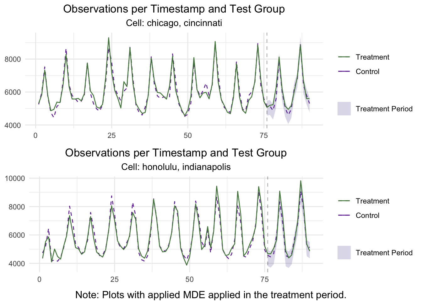
Moreover, we could plot these results to observe how the model fits the historical data.
plot(Markets,
     test_markets = test_locs,
     type = "Lift",
     stacked = TRUE)
3. Detailed Power Curves
Perhaps the most important piece of part of any Market Selection process is to obtain and analyze the test's Power Curve. These curves tell us how sensible our test is at detecting a given Lift, it's statistical power, and give us a good estimate of the necessary budget needed to run the Multi-Cell test. The MultiCellPower function can be used to calculate the Power Curves for a given set of cells through simulations on the historical data.
The MultiCellPower function is very easy to use as it will leverage the set-up and results we obtained from MultiCellMarketSelection. The most important parameters to calculate the Power Curves are:
x: AMultiCellMarketSelectionobject.test_markets: A list of the selectedmarket_IDpercell_ID. It is important to make sure that this list contains exactlyknumeric values corresponding to the results ofMultiCellMarketSelection. The recommended layout islist(cell_1 = 1, cell2 = 1, cell3 = 1,...), for our example we will set it to the previously defined list:test_locs.effect_size: This parameter contains the different Lifts that we will simulate for our test. For each value in this parameter, the algorithm will simulate a GeoLift test with that Lift and will assess the statistical significance of the results to determine the test's Statistical Power. For this parameter, it is important to make sure that the sequence includes zero. For our example, we will set both positive and negative effect sizes to observe the curve's form and to see how symetrical it is.lookback_window: This parameter indicates how long back in history the simulations will go. Setting alookback_windowto a value greater than one is particularly important to correctly assess the Power and estimate the budget of tests with significant seasonality or which aren't very stable. For this example, we will simulate an entire week, thuslookback_window = 7.side_of_test: Indicates whether aone_sidedortwo_sidedtest will be performed. The function will use the same value used forMultiCellMarketSelectionunless specified otherwise. In this example, we will leave this parameter blank so it will default to the value specified in the previous step (one_sided).
Power <- MultiCellPower(Markets,
                        test_markets = test_locs,
                        effect_size =  seq(-0.5, 0.5, 0.05),
                        lookback_window = 7)
Plotting the results shows the Power Curve for each cell.
plot(Power,
     actual_values = TRUE,
     smoothed_values = FALSE,
     show_mde = TRUE,
     breaks_x_axis = 15,
     stacked = TRUE)
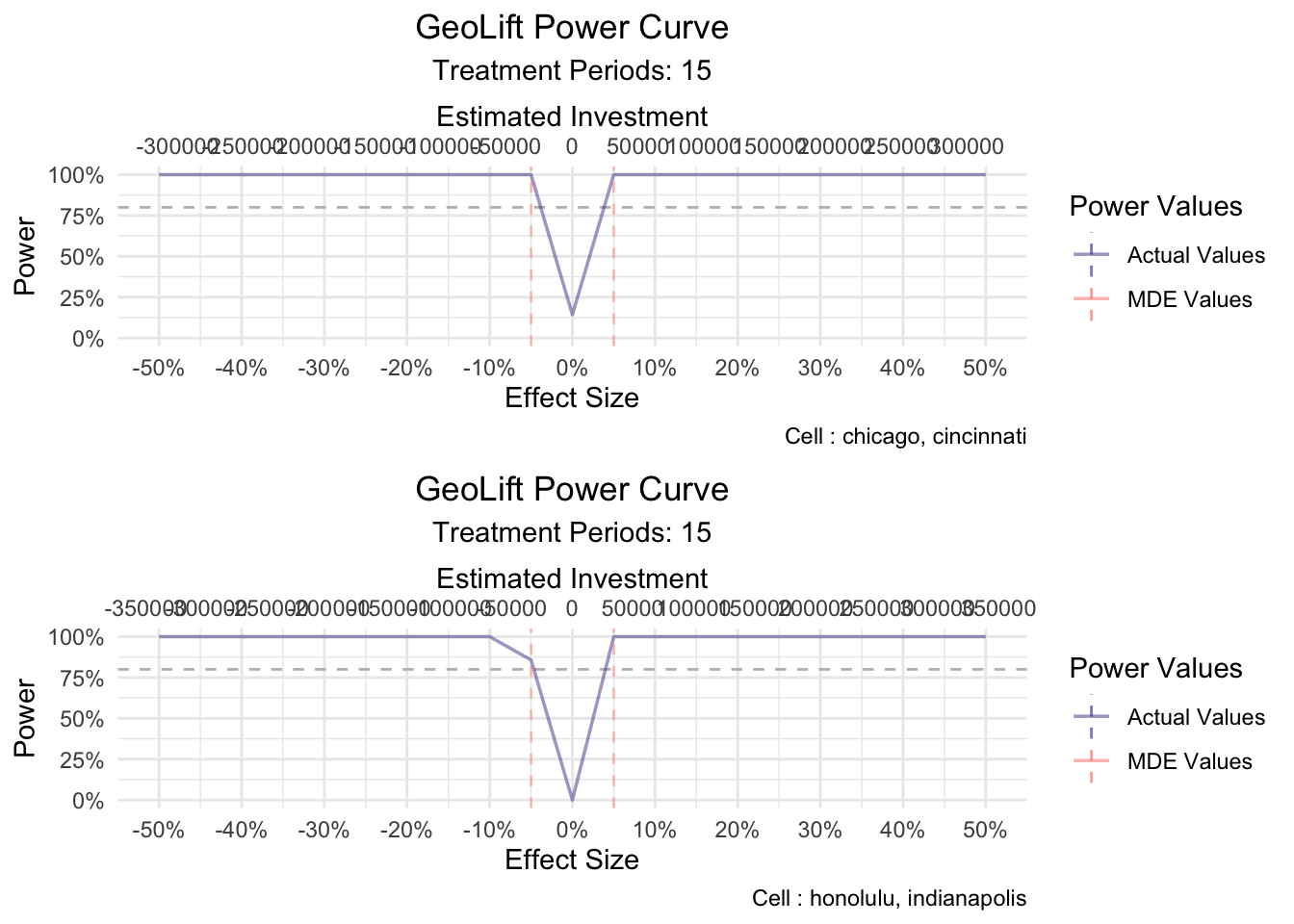
The plot shows that both Power Curves are ideal as they are: symmetric, centered at zero, and have relatively small effect sizes needed to accurately detect lift (~5%). Moreover, we observe that, despite different cpics, an investment of $50,000 per cell should be more than enough to achieve a significant Lift.
[Optional]: MultiCellWinner
While most of the times the objective of a Multi-Cell test is simply to accurately measure the incremental effect of different channels/strategies, sometimes we want to go a step further and declare which one of the competing cells is statistically significantly better or worse than the others. In this case, we can use the MultiCellWinner function, to determine what must happen for a cell to be declared a "Winner". This function works by answering the following question: for a given baseline Effect Size, how much better must the incremental Return on Ad Spend (iROAS) of a cell be so that it provides a statistically significantly better Lift overall?
The most important parameters of the MultiCellWinner function are:
x: AMultiCellPowerobject created by theMultiCellPowerfunction. By using this object, the winner analysis will be conducted on the cells defined previously. Specifically, Cell 1: Chicago and Cincinnati and Cell B: Honolulu and Indianapolis.effect_size: A numeric value representing the Lift that will be simulated across all cells. If not specified (default), the algorithm will use the largest lift found inMultiCellPowerthat provides a well-powered test across all cells. For this example, we will se the baseline Lift at 10%.geolift_type: Specifies the type of GeoLift test to be performed which can be: "standard" (test regions will receive the treatment) or "inverse" (test regions will be holded-out from the treatment). More information on standard and inverse tests can be found here.ROAS: Provides a series of incremental Return on Ad Spend (iROAS) values to assess. In this example we will use ROAS that range from 1x to 10x increasing by 0.5x through the sequence:seq(1,10,0.5).alpha: Significance Level. By default 0.1.method: This parameter indicates the mathematical method used to calculate the aggregate ATT Confidence Intervals. The user can choose between "conformal" (recommended) and "jackknife+".stat_test: Indicates the stat test that will be used in our calculations. This parameter can take the values of "Total", "Negative", or "Positive". For this example, we will set this parameter to "Positive" as we conducted a Standard GeoLift Multi-Cell test.
Winners <- MultiCellWinner(Power,
                           effect_size = 0.1,
                           geolift_type = "standard",
                           ROAS = seq(1,10,0.5),
                           alpha = 0.1,
                           method = "conformal",
                           stat_test = "Positive"
)
Winners
##                cell_A incremental_A lowerCI_Cell_A upperCI_Cell_A
## 1 chicago, cincinnati      78534.65        76612.9         557051
##                   cell_B incremental_B lowerCI_Cell_B upperCI_Cell_B duration
## 1 honolulu, indianapolis      9065.861        3467.71        75443.9       15
##   ROAS
## 1    9
These results show that Cell 1 would need to be 9x more effective than Cell 2 to be declared a "Winner".
4. Campaign Execution
After successfully selecting the test markets with MultiCellMarketSelection and GeoLiftPower, the campaigns can be executed. For this test we will run ads on Social Media for the cities of Chicago and Cincinnati (Cell 1), Paid Search ads for the cities of Honolulu and Indianapolis (Cell 2), and holdout the rest of the locations in our data-set for a 15-day test.
We can use the simulated Multi-Cell data included in the GeoLift package as follows:
data(GeoLift_Test_MultiCell)

# Read test data
GeoTestData_Test <- GeoDataRead(data = GeoLift_Test_MultiCell,
                                    date_id = "date",
                                    location_id = "location",
                                    Y_id = "Y",
                                    X = c(), #empty list as we have no covariates
                                    format = "yyyy-mm-dd",
                                    summary = TRUE)

## ##################################
## #####       Summary       #####
## ##################################
##
## * Raw Number of Locations: 40
## * Time Periods: 105
## * Final Number of Locations (Complete): 40
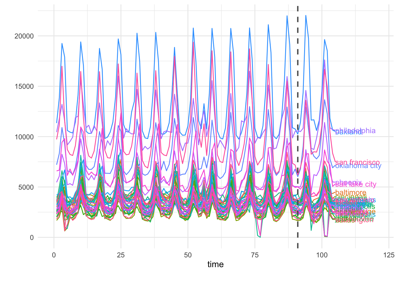
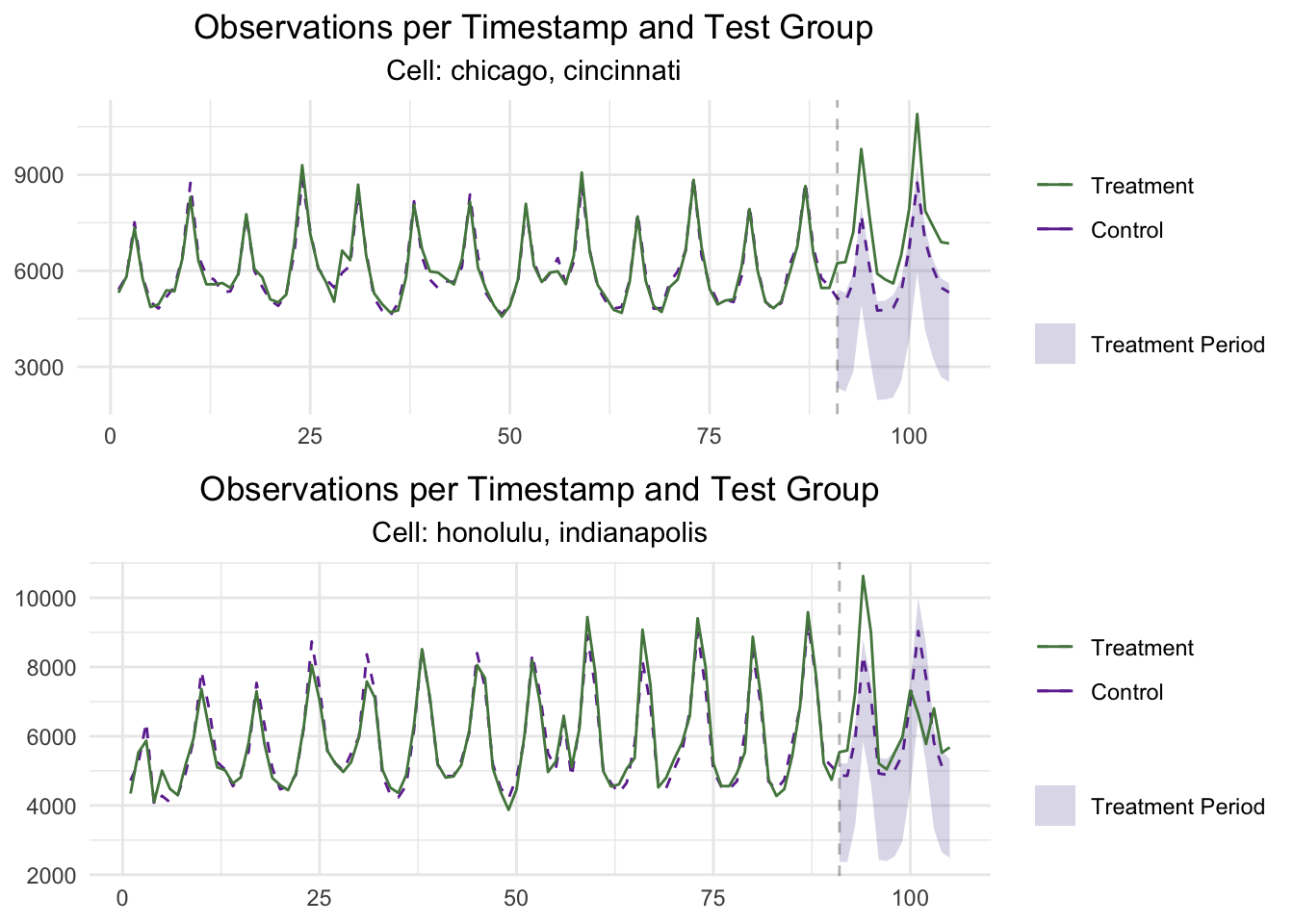
# Plot the historical and test data
GeoPlot(GeoTestData_Test,
        treatment_start = 91)
5. Multi-Cell Inference for GeoLift
The final step in the process is to calculate the Lift generated by our Social Media and Paid Search campaigns. We can leverage the GeoLiftMultiCell function to easily perform statistical inference on our test. The key parameters of this function are:
data: A data.frame containing the historical conversions by geographic unit. It requires at least a "locations" column with the geo name, a "Y" column with the outcome data (units), a time column with the indicator of the time period (starting at 1), and covariates (optional). In this example, we will use theGeoTestData_Testdata frame we just obtained throughGeoDataRead.locations:A list of lists of test markets per cell. The recommended layout islist(cell_1 = list("locA"), cell2 = list("locB"), cell3 = list("locC"),...).treatment_start_time: Time index of the start of the treatment. 91 for this example.treatment_end_time: Time index of the end of the treatment. 105 for this example.alpha: Significance level. Set to 0.1 by default.model: This parameter indicates which (if any) prognostic function will be used to augment our Augmented Sythetic Control Method (ASCM). The available options for this parameter are: "None", "Ridge", "GYSN", and "best". We will set this parameter to "best" to let the algorithm determine the optimal prognostic function.fixed_effects: Indicates whether to include a Fixed Effects component in the model or not. Given our prior knowledge of this simulated data, we will set it toTRUE.ConfidenceIntervals: Indicates whether to estimate the Confidence Intervals for the total Lift.method: Identifies the mathematical methodology that will be used to calculate our Confidence Intervals. We will set this parameter to the recommended option which is "conformal".geolift_type: String that specifies the type of GeoLift test to be performed. This parameter can be set to: "standard" or "inverse". Given that this was a "standard" Multi-Cell GeoLift test, we will set this parameter accordingly.stat_test: Determines the test statistic to be used by GeoLift. Valid options are: "Total", "Negative", and "Positive". We will use the latter as this was a standard GeoLift Multi-Cell test.winner_declaration: Logic flag indicating whether to compute a winner cell analysis. If set to TRUE (default), both pairwise and total statistical significance tests will be performed.
# First we specify our test locations as a list
test_locations <- list(cell_1 = list("chicago", "cincinnati"),
                       cell_2 = list("honolulu", "indianapolis"))

#Then, we run MultiCellResults
MultiCellResults <- GeoLiftMultiCell(data = GeoTestData_Test,
                                     locations = test_locations,
                                     treatment_start_time = 91,
                                     treatment_end_time = 105,
                                     alpha = 0.1,
                                     model = "best",
                                     fixed_effects = TRUE,
                                     ConfidenceIntervals = TRUE,
                                     method = "conformal",
                                     stat_test = "Positive",
                                     winner_declaration = TRUE)

## Selected Ridge as best model.
## Selected Ridge as best model.
##
## ##################################
## ##### Pairwise  Comparisons #####
## ##################################
##                Cell_A  Lower_A   Upper_A                 Cell_B Lower_B
## 1 chicago, cincinnati 16673.88 146162.26 honolulu, indianapolis 8745.23
##     Upper_B Winner
## 1 118669.62   <NA>
MultiCellResults

## ##################################
## #####     Cell 1 Results    #####
## ##################################
## Test results for 15 treatment periods, from time-stamp 91 to 105 for test markets:
## 1 CHICAGO
## 2 CINCINNATI
## ##################################
## #####     Test Statistics    #####
## ##################################
##
## Percent Lift: 22.8%
##
## p-value: 0
##
## Incremental Y: 20215
##
## Average Estimated Treatment Effect (ATT): 673.819
##
## The results are significant at a 95% level. (ONE-SIDED POSITIVE LIFT TEST)
##
## There is a 0% chance of observing an effect this large or larger assuming treatment effect is zero.
## ##################################
## #####     Cell 2 Results    #####
## ##################################
## Test results for 15 treatment periods, from time-stamp 91 to 105 for test markets:
## 1 HONOLULU
## 2 INDIANAPOLIS
## ##################################
## #####     Test Statistics    #####
## ##################################
##
## Percent Lift: 7.1%
##
## p-value: 0
##
## Incremental Y: 6493
##
## Average Estimated Treatment Effect (ATT): 216.423
##
## The results are significant at a 95% level. (ONE-SIDED POSITIVE LIFT TEST)
##
## There is a 0% chance of observing an effect this large or larger assuming treatment effect is zero.
The results show that the Social Media campaign had a significant Lift equal to 22.8% while the Paid Search campaigns generated a 7.1% Lift. And while the results of the test show a higher Lift by Cell 1, the wide Confidence Intervals do not allow us to declare a winner at a 90% confidence level. We can dig deeper into the results through the summary() of our Multi-Cell GeoLift object. The summary() method has two options based on the table parameter:
- If
table = TRUEa summary table of the results per cell will be printed.
#Short summary of the results
summary(MultiCellResults, table = TRUE)

## | Cell|Location               | Duration|Lift  | Incremental|     ATT| pValue|Stat_Test                    | Stat_Sig|Prognostic_Func |Winner |
## |----:|:----------------------|--------:|:-----|-----------:|-------:|------:|:----------------------------|--------:|:---------------|:------|
## |    1|CHICAGO, CINCINNATI    |       15|22.8% |       20215| 673.819|      0|ONE-SIDED POSITIVE LIFT TEST |        1|RIDGE           |       |
## |    2|HONOLULU, INDIANAPOLIS |       15|7.1%  |        6493| 216.423|      0|ONE-SIDED POSITIVE LIFT TEST |        1|RIDGE           |       |
- If
table = FALSEthe complete summary method for each cell will be outputted.
# Deep dive into the results
summary(MultiCellResults, table = FALSE)

## ##################################
## #####     Cell 1 Results    #####
## ##################################
##
## GeoLift Results Summary
## ##################################
## #####     Test Statistics    #####
## ##################################
##
## * Average ATT: 673.819
## * Percent Lift: 22.8%
## * Incremental Y: 20215
## * P-value: 0
## * 90% Confidence Interval: (16673.879, 146162.255)
##
## ##################################
## #####   Balance Statistics   #####
## ##################################
##
## * L2 Imbalance: 956.678
## * Scaled L2 Imbalance: 0.1694
## * Percent improvement from naive model: 83.06%
## * Average Estimated Bias: -0.441
##
## ##################################
## #####     Model Weights      #####
## ##################################
##
## * Prognostic Function: RIDGE
##
## * Model Weights:
##  * portland: 0.2121
##  * austin: 0.1521
##  * nashville: 0.1463
##  * san diego: 0.1371
##  * minneapolis: 0.1364
##  * new york: 0.06
##  * baton rouge: 0.0558
##  * reno: 0.0474
##  * miami: 0.0359
##  * atlanta: 0.0118
##  * houston: 0.0044
##  * san antonio: 0.0041
##  * salt lake city: -0.0013
##  * oakland: -8e-04
##  * philadelphia: -7e-04
##  * oklahoma city: -4e-04
##  * baltimore: 2e-04
##  * las vegas: 2e-04
##  * dallas: 2e-04
##  * new orleans: -1e-04
##  * san francisco: -1e-04
##  * boston: -1e-04
##  * columbus: 1e-04
##  * washington: -1e-04
##  * kansas city: -1e-04
##  * phoenix: -1e-04
##  * memphis: -1e-04
##  * milwaukee: -1e-04
##  * cleveland: -1e-04
##  * saint paul: 1e-04
##
## ##################################
## #####     Cell 2 Results    #####
## ##################################
##
## GeoLift Results Summary
## ##################################
## #####     Test Statistics    #####
## ##################################
##
## * Average ATT: 216.423
## * Percent Lift: 7.1%
## * Incremental Y: 6493
## * P-value: 0
## * 90% Confidence Interval: (8745.226, 118669.618)
##
## ##################################
## #####   Balance Statistics   #####
## ##################################
##
## * L2 Imbalance: 1508.472
## * Scaled L2 Imbalance: 0.326
## * Percent improvement from naive model: 67.4%
## * Average Estimated Bias: 11.782
##
## ##################################
## #####     Model Weights      #####
## ##################################
##
## * Prognostic Function: RIDGE
##
## * Model Weights:
##  * austin: 0.3567
##  * tucson: 0.2351
##  * portland: 0.1744
##  * nashville: 0.0988
##  * baton rouge: 0.0823
##  * detroit: 0.0445
##  * orlando: 0.0391
##  * phoenix: -0.0136
##  * columbus: -0.0129
##  * salt lake city: -0.0125
##  * memphis: -0.0106
##  * oklahoma city: 0.0102
##  * miami: -0.0093
##  * houston: 0.0073
##  * las vegas: -0.007
##  * baltimore: -0.0066
##  * san francisco: -0.006
##  * jacksonville: 0.006
##  * kansas city: 0.0054
##  * milwaukee: 0.0043
##  * cleveland: 0.0042
##  * philadelphia: 0.0041
##  * denver: -0.0032
##  * new orleans: -0.0028
##  * los angeles: 0.0023
##  * washington: 0.0023
##  * minneapolis: 0.002
##  * san diego: 0.0017
##  * dallas: 0.0016
##  * san antonio: 0.0014
##  * reno: 0.0014
##  * atlanta: -0.0013
##  * boston: 0.0013
##  * new york: -9e-04
##  * oakland: 6e-04
##  * saint paul: -1e-04
##
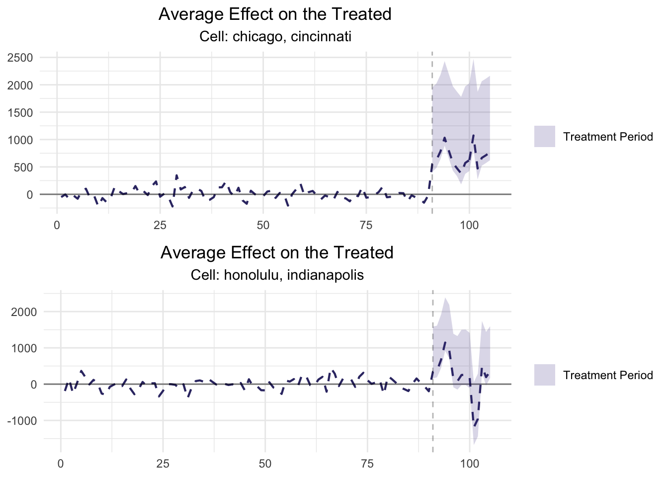
Finally, we can plot the results to observe both the Lift and ATT plots.
plot(MultiCellResults, type = "Lift", stacked = TRUE)
plot(MultiCellResults, type = "ATT", stacked = TRUE)