Enter into the time capsule - Determining Lookback Window

“Aunque me fuercen yo nunca voy a decir

Que todo tiempo, por pasado fue mejor"

- Luis Alberto Spinetta

TL;DR

• The success of a geo-based experiment greatly depends on the Market Selection process.
• In the GeoLift package, we use historical data and a simulation-based approach to identify the best set of treatment and control locations based on the constraints specified by the user.
• Selecting an appropriate value for the lookback_window parameter (the amount of pre-treatment periods that will be considered) is a very important part of the process.
• Based on the analysis presented in this note, we generally recommend using 1/10th of the pre-treatment period as a simulation lookback_window (especially if your time-series has a lot of variability across time).

What is considered a simulation in GeoLift?

Essentially, before running the actual test, we are running a series of geo experiments to determine which is the best setup that will pave the way to success. As explained in further detail in our Blueprint Course, the GeoLift Market Selection process simulates a large number of geo experiments to determine which is the best test and control setup for you.

In each simulation a treatment effect is applied over a treatment group during the treatment period. Then, GeoLift then trains a counterfactual for the treatment group by using all of the pre-treatment periods prior to the experiment to assess the model's performance. Let’s breakdown each of these five components:

• The treatment effect: is the Lift percentage that will be applied to a set of locations during the testing period.
• The treatment group: these are a set of locations that will be exposed to the treatment effect.
• The counterfactual: these are a set of locations that are used to estimate what would have happened to the treatment group if it had not been exposed to the treatment effect. An easy way to think about it is as a weighted average of all the locations that are not part of the treatment group.
• The treatment period: represents the moments in which the treatment group will be exposed to the treatment.
• The pre-treatment period: this refers to the amount of periods that will be used to build the counterfactual, where there was no simulated difference between locations. During this period, the counterfactual and the treatment group should have a similar behavior.

Applying different effects to the same group in the same period allows us to holistically determine what the Minimum Detectable Effect (MDE) for that setup will be. Among other metrics, this helps us understand whether we are dealing with a combination of locations that will have a higher likelihood of observing small effect sizes. However, seasonalities and variations throughout time make can difficult to estimate the MDE with complete certainty. Fortunately, we can reduce this uncertainty by taking a look at the past!

Introducing the lookback window parameter.

Our first simulation uses the most recent/latest periods in our series as our treatment period and all of the remaining periods as our pre-treatment period. This gives us the metrics we need to rank treatment groups for those time periods.

As stated in our GeoLift Walkthrough, we can increase the number of simulated time periods by changing the lookback_window. The lookback_window indicates how far back in time the simulations for the power analysis will go. By increasing the lookback_window, we subtract the last period from the previous simulation’s total duration and repeat the process over the remaining periods. Finally, we calculate the average metrics for each treatment group over all of the runs in different periods.

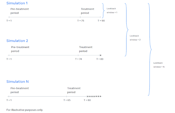
For example, imagine we have a 90 day long series with different locations and we would like to simulate a 15 day test, with a 2 day lookback_window.

• In the first simulation, the treatment period is made up of the most recent dates and Lift is simulated on it. The remainder, the pre-treatment period, is used to build a counterfactual. So, with a test duration of 15 days, for this iteration we use periods 1 to 75 as a pre-treatment period and periods 76 to 90 as a treatment period.
• For our second simulation, the treatment period is shifted by one timestamp. We use periods 1 to 74 as a pre-treatment period and periods 75 to 89 as a treatment period.
• We then construct average metrics per each treatment group, using these two simulations. In essence, we are repeating this flow until the number of time periods shifted is equal to the lookback_window parameter.

In this context, more simulations allow us to have a more robust estimate of the metrics for each treatment group, observing if the same behavior occurs across different simulated treatment and pre-treatment periods. The intuitive idea here is that we would like to capture some of the variability in the time series in our test setups, to avoid assuming something that could be different in the future.

There’s a tradeoff: robustness vs preciseness

The more we look back into the past, the more simulations per treatment group we will have. This will make our estimates more robust and allow us to make safer predictions with regard to the pre-test metrics.

However, the more we look back into the past, the less precise our simulation will be as compared to the actual result. Removing the last periods we have prior to the test leads to two major effects:

• Our simulations become less precise because they have a smaller amount of periods to build the counterfactual than what the actual experiment will have.
• The accuracy of our simulation will be reduced since we are shortening the time that is being considered by the algorithm’s pre-treatment period.

Given this tradeoff, we need to choose the amount of simulations we run considering the potential they have but keeping in mind that they also have a downside. Moreover, it is important to note that incresing the lookback_window parameter will exponentially increase the number of simulations performed in the Market Selection algorithm and will result in a longer runtime.

How to choose the best lookback_window?

The best way to analyze this problem is to capture the variance of detected effects in the same simulated treatment period for different treatment group combinations.

We have run this analysis using the dummy dataset that is available within the GeoLift package (data(GeoLift_PreTest)). This dataset is similar to the example we showed above: it has a total of 90 days of pre-experiment data, and we will simulate a test that will last 15 days. If we assume that there was no preexisting difference between locations, then the median of detected effects for each test start period should be around zero, which is the true effect.

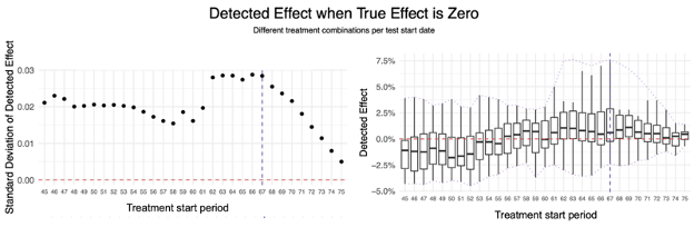
The plot on the left shows the standard deviation of the detected effect per treatment start period. The plot on the right shows the range of detected effects for different treatment groups.

As we can see from the plot in the left, the standard deviation of the detected effect has a continuous drop from period 67 onwards. From the second plot, we can also observe that the median effect is close to zero, especially in the last periods.

Putting it in practice

Since we have 75 pre-treatment periods in total, and the drop in standard deviation occurs in period 67, we would set a lookback_window of 8 periods.

To be as efficient as possible, we suggest running the GeoLiftMarketSelection function to find the best combination of markets with a lookback_window=1. With those best candidates, do a deep dive with a longer lookback_window=8 for each treatment combination by running GeoLiftPower, plot and analyze their power curves.

In conclusion

The lookback_window parameter is a fundamental element of a robust Power Analysis and Market Selection. As a best practice, we recommend running a data-driven analysis similar to the one that was showcased here to identify the ideal value for this parameter. Alternatively, a great rule of thumb is to keep 1/10 of the pre-treatment periods for simulations, once the test duration has been defined. So, if you have a total of 150 periods before your experiment, and you want to run a 10 day test, a total of 140 pre-treatment periods would remain. Following this rule, you would have to set a lookback_window=14 for the preferred options that come out of the GeoLiftMarketSelection ranking.

At the very least, we suggest setting the lookback_window to a value that is at least as large as the time-series’ most granular seasonality (if we observe that sales vary widely throughout the days of the week, then setting the lookback_window to 7 would be a good start).

What’s up next?

Stay tuned for our next blog posts, related to topics like:

• When should I use Fixed Effects to get a higher signal to noise ratio?
• When should our GeoLift test start?