One post tagged with "continuous lift"

TL;DR​

• This blog post demonstrates how to deal with treated observations in sequential GeoLift testing.
• Currently, when running two sequential GeoLifts, the treatment period of the first experiment becomes part of the pre-treatment period of the second experiment, potentially affecting results and power calculations.
• To prevent this, you can replace the treatment locations in the first experiment with the best counterfactual available. Once the treatment location has been replaced, make sure to expand the control donor pool with said series.
• We introduce our ReplaceTreatmentSplit function to replace the treated location units, easily implementing our proposed solution.

Introduction​

Advertisers have many questions to answer like, “What’s the incremental impact of this media channel?” and “What’s the budget elasticity of my investment in this channel?”. These questions and more can be answered using GeoLift.

Since each question is different and we cannot answer them all at the same time, we need to decide which of them we should answer first by building a learning agenda. Our agenda holds everything from business questions and hypotheses to specific experiment designs that will give us the answers we are looking for. For the sake of simplicity, imagine we have two business questions, and we run our first GeoLift (experiment 1) to answer the first one and would like to design a new GeoLift (experiment 2) to give an answer to our second inquiry.

However, running a second GeoLift immediately after the previous one is not that simple.

Sequential GeoLift testing​

At a first glance, we have a couple of options:

Option 1: Repeating our experiment 1 treatment group in experiment 2, excluding the experiment 1 periods.​

This implies that we will remove experiment 1 time periods from the pre-treatment period, meaning we will get the same time series we had before experiment 1 was run. Furthermore, if we rerun the power analysis with this series, we will get the same treatment group we had for experiment 1.

While an attractive option, it lacks flexibility due to the fact that we will probably choose the same treatment we did before experiment 1. Furthermore, we should make sure that the GeoLift model is able to accurately predict the most recent time-stamps, using the latest market dynamics. For example, if we had a test for all of December, then the model trained up to November might struggle to predict January due to different spending trends. Moreover, if the treatment was very long, this might make it very hard to justify tying the set of pre-treatment periods for experiment 1 to the periods during experiment 2.

Option 2: Rerunning the power analysis for experiment 2, without excluding experiment 1 periods.​

Without removing the periods from experiment 1, we will preserve the autocorrelation within the time series and avoid the sudden change that may occur, while keeping the latest time-stamps. Having said this, going with this option poses another threat. Locations that were used as a treatment group in experiment 1 will probably not be chosen as a good setup in the GeoLift ranking algorithm. When we run simulations using those locations, the simulated effect will probably be far off from the observed effect, since they already had a previous treatment that we are not considering.

If the locations selected as the treatment group presented a good setup for experiment 1, then at least some of them should be selected to be part of the treatment of experiment 2.

Our solution: Replace treatment group values from experiment 1​

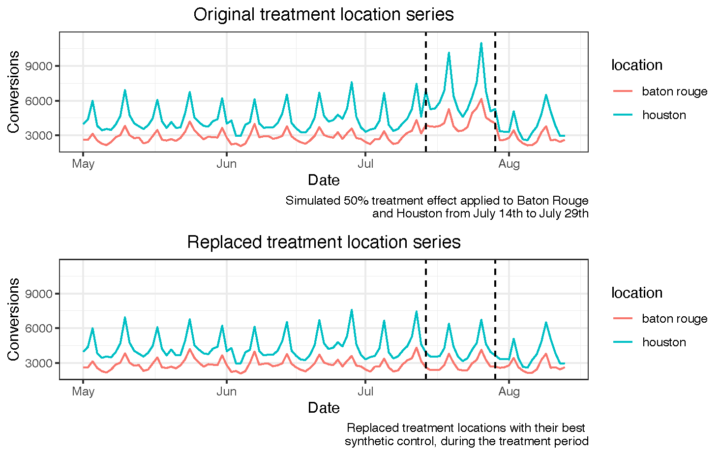
Our goal is maximizing the amount of data we have without excluding any periods and guaranteeing that our dataset does not contain any structural changes (treatment applied to certain locations in experiment 1). To do so, we recommend replacing the values of the locations that were treated during experiment 1, during the periods in which the treatment occurred and including them in the control donor pool. For reference, here’s a picture of what this looks like.

Here’s an example of our pseudo-code:

1. Define locations that were treated and treatment period during experiment 1.
2. Fit a GeoLift counterfactual to each of the treatment locations, training it on experiment 1’s pre-treatment period.
3. Only keep the counterfactual that has the closest match to a treatment location in the pre-treatment period (using absolute L2 imbalance, A.K.A. the sum of squared differences between treatment and control prior to the experiment).
4. Replace the selected treatment location by its counterfactual values during the experiment 1’s treatment period.
5. Reassign the replaced treatment location to the control donor pool.
6. Repeat this process until there are no more treatment locations left.

This solution has three clear benefits:

• We preserve the time series structure without excluding any data.
• We replace the structural change in the treatment locations by our best estimate of what would have happened if they had not been treated.
• We have a higher chance of providing better counterfactual fits for the replaced treatments because we are enlarging the control donor pool with each replacement.

Data-driven validation​

The last of these benefits does not necessarily mean that we will always be better off. Particularly, the algorithm will provide the same L2 imbalance values for cases where we have a smaller treatment size given that the added value of the replaced treatment to the control donor pool will not be as large.

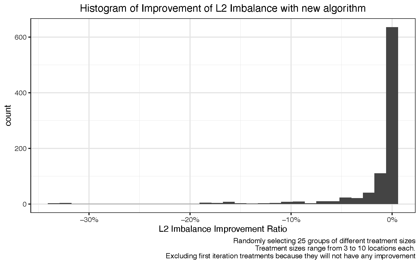
In order to understand what was the average impact that our algorithm had on L2 imbalance, we decided to run a random selection of locations to build different treatment groups of 5 locations. We then passed those random groups through the algorithm, and compared it to the L2 imbalance that the counterfactual would have if the replaced treatment had not been added to the control donor pool. That is what we call the L2 imbalance improvement ratio:

While the majority of the observations for the L2 imbalance improvement ratio are close to zero, there is a negative long tail that shows that there are some cases where our algorithm works better than the alternative.

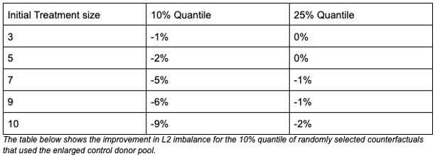
To make our finding more robust, we repeated the simulations with randomly selected treatment groups of different sizes. Looking at the 10% and 25% quantiles of the histogram provided above for each treatment size, we saw improvements in L2 imbalance of up to 8% in the 10% quantile. Naturally, the larger the treatment group, the higher the benefit of our proposed solution, in line with our aforementioned hypothesis.

How to implement the algorithm?​

We have recently landed a simple method for you to use if you would like to leverage this algorithm. Simply implement the ReplaceTreatmentSplit function, specifying what the treatment locations and the treatment start date and end date for experiment 1 are. You can pick up the replaced dataset from the $data argument in the list. The $l2_imbalance_df will give you the data frame of L2 imbalances for each treatment location when they were replaced.

# Import libraries and transform data.
library(GeoLift)
data(GeoLift_Test)
geo_data <- GeoDataRead(data = GeoLift_Test,
                        date_id = "date",
                        location_id = "location",
                        Y_id = "Y",
                        X = c(), #empty list as we have no covariates
                        format = "yyyy-mm-dd",
                        summary = TRUE)
treatment_group <- c(‘chicago’, ‘portland’)

# Replace treatment locations for best counterfactual.
g <- ReplaceTreatmentSplit(
  treatment_locations = treatment_group,
  data = geo_data,
  treatment_start_time = 90,
  treatment_end_time = 105,
  model = "none",
  verbose = TRUE
)

# Extract replaced data.
new_geo_data <- g$data

What’s up next?​

Keep your eye out for our coming blog posts, around topics like:

• When should I use Fixed Effects to get a higher signal to noise ratio?
• Long term branding measurement with GeoLift.